4.2 Histograms and Frequencies
A histogram tabulates counts and frequencies of observed data over a set of contiguous intervals. Let \(b_{0}, b_{1}, \cdots, b_{k}\) be the breakpoints (end points) of the class intervals such that \(\left(b_{0}, b_{1} \right], \left(b_{1}, b_{2} \right], \cdots, \left(b_{k-1}, b_{k} \right]\) form \(k\) disjoint and adjacent intervals. The intervals do not have to be of equal width. Also, \(b_{0}\) can be equal to \(-\infty\) resulting in interval \(\left(-\infty, b_{1} \right]\) and \(b_{k}\) can be equal to \(+\infty\) resulting in interval \(\left(b_{k-1}, +\infty \right)\). Define \(\Delta b_j = b_{j} - b_{j-1}\) and if all the intervals have the same width (except perhaps for the end intervals), \(\Delta b = \Delta b_j\). To count the number of observations that fall in each interval, we can use the count function: \[ c(\vec{x}\leq b) = \#\lbrace x_i \leq b \rbrace \; i=1,\ldots,n \] \(c(\vec{x}\leq b)\) counts the number of observations less than or equal to \(x\). Let \(c_{j}\) be the observed count of the \(x\) values contained in the \(j^{th}\) interval \(\left(b_{j-1}, b_{j} \right]\). Then, we can determine \(c_{j}\) via the following equation: \[ c_{j} = c(\vec{x}\leq b_{j}) - c(\vec{x}\leq b_{j-1}) \] The key parameters of a histogram are:
- The first bin lower limit (\(b_{0}\)): This is the starting point of the range over which the data will be tabulated.
- The number of bins (\(k\)))
- The width of the bins, (\(\Delta b\))

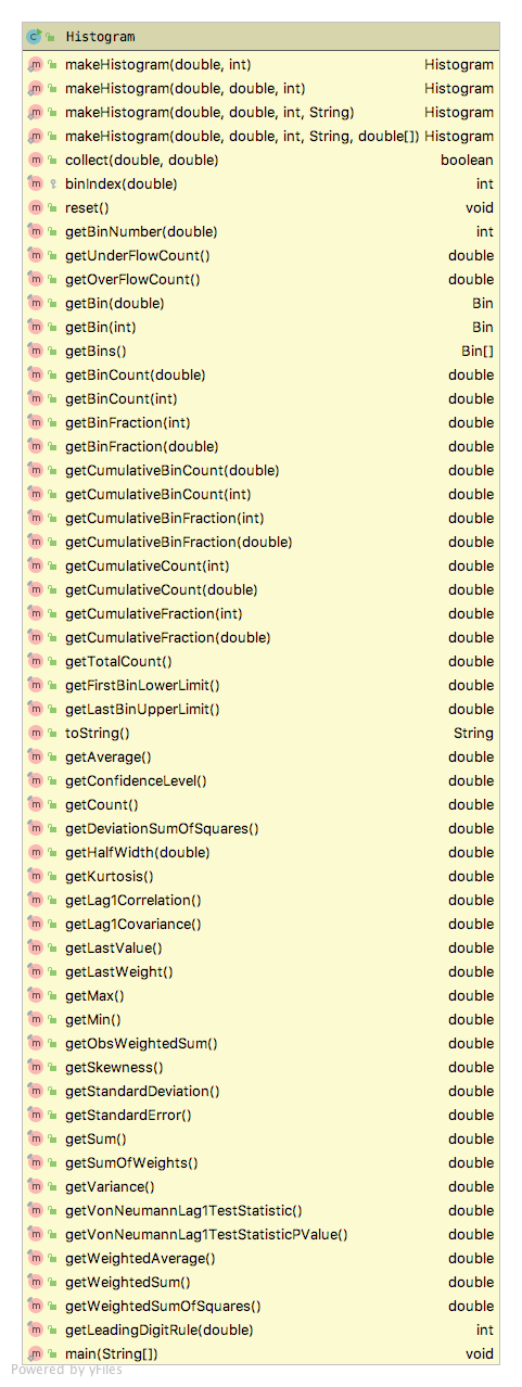
Figure 4.4: Histogram Class
Figure 4.4 presents the methods of the Histogram class. The Histogram class is utilized in a very similar manner as the Statistic class by collecting observations. The observations are then tabulated into the bins. The Histogram class allows the user to tabulate the bin contents via the collect() methods inherited from the AbstractStatistic base class. Since data may fall below the first bin and after the last bin, the implementation also provides counts for those occurrences. Since a Histogram is a sub-class of AbstractStatistic, it also implements the StatisticAccessorIfc to provide summary statistics on the data tabulated within the bins. The Histogram class also provides static methods to create histograms based on a range (lower limit to upper limit) with a given number of bins. In this case, an appropriate bin width is computed.
In some cases, the client may not know in advance the appropriate settings for the number of bins or the width of the bins. In this situation, one can use the CachedHistogram class, which first collects the data in a temporary cache array. Once the cache has been filled up, the CachedHistogram computes a reasonable lower limit, number of bins, and bin width based on the statistics collected over the cache. The underlying histogram is available via the getHistogram() method after the cache has been used.
ExponentialRV d = new ExponentialRV(2);
// create a histogram with lower limit 0.0, 20 bins, of width 0.1
Histogram h = new Histogram(0.0, 20, 0.1);
for (int i = 1; i <= 100; ++i) {
    h.collect(d.getValue());
}
System.out.println(h);
Histogram: Histogram
-------------------------------------
Number of bins = 20
Bin width = 0.1
First bin starts at = 0.0
Last bin ends at = 2.0
Under flow count = 0.0
Over flow count = 45.0
Total bin count = 55.0
Total count = 100.0
-------------------------------------
Bin Range Count Total Prob CumProb
1 [0.00,0.10) 2.0 2.0 0.036364 0.036364
2 [0.10,0.20) 5.0 7.0 0.090909 0.127273
3 [0.20,0.30) 5.0 12.0 0.090909 0.218182
4 [0.30,0.40) 2.0 14.0 0.036364 0.254545
5 [0.40,0.50) 7.0 21.0 0.127273 0.381818
6 [0.50,0.60) 3.0 24.0 0.054545 0.436364
7 [0.60,0.70) 3.0 27.0 0.054545 0.490909
8 [0.70,0.80) 3.0 30.0 0.054545 0.545455
9 [0.80,0.90) 2.0 32.0 0.036364 0.581818
10 [0.90,1.00) 2.0 34.0 0.036364 0.618182
11 [1.00,1.10) 5.0 39.0 0.090909 0.709091
12 [1.10,1.20) 6.0 45.0 0.109091 0.818182
13 [1.20,1.30) 2.0 47.0 0.036364 0.854545
14 [1.30,1.40) 2.0 49.0 0.036364 0.890909
15 [1.40,1.50) 3.0 52.0 0.054545 0.945455
16 [1.50,1.60) 1.0 53.0 0.018182 0.963636
17 [1.60,1.70) 1.0 54.0 0.018182 0.981818
18 [1.70,1.80) 1.0 55.0 0.018182 1.000000
19 [1.80,1.90) 0.0 55.0 0.000000 1.000000
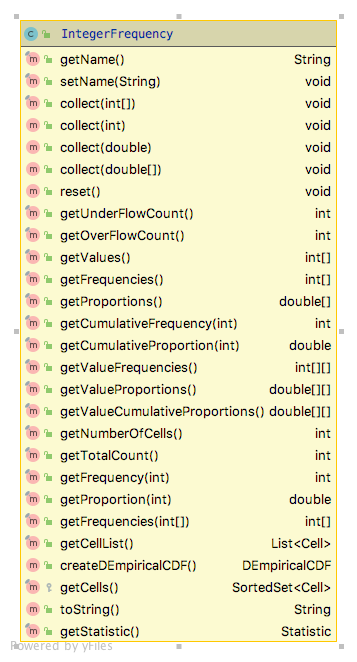
20 [1.90,2.00) 0.0 55.0 0.000000 1.000000 The JSL will also tabulate count frequencies when the values are only integers. This is accomplished with the IntegerFrequency class. Figure 4.5 indicates the methods of the IntegerFrequency class. The object can return information on the counts and proportions. It can even create a DEmpiricalCDF distribution based on the observed data.

Figure 4.5: IntegerFrequence Class
In the following code example, an instance of the IntegerFrequency class is created. Then, an instance of a binomial random variable is used to generate a sample of 10,000 observations. The sample is then collected by the IntegerFrequency class’s collect() method.
IntegerFrequency f = new IntegerFrequency("Frequency Demo");
BinomialRV bn = new BinomialRV(0.5, 100);
double[] sample = bn.sample(10000);
f.collect(sample);
System.out.println(f);
As can be noted in the output, only those integers that are actually observed are tabulated in terms of the count of the number of times the integer is observed and its proportion. The user does not have to specify the range of possible integers; however, instances of IntegerFrequency can be created that specify a lower and upper limit on the tabulated values. The overflow and underflow counts then tabulate when observations fall outside of the specified range.
Frequency Tabulation Frequency Demo
----------------------------------------
Number of cells = 39
Lower limit = -2147483648
Upper limit = 2147483647
Under flow count = 0
Over flow count = 0
Total count = 10000
----------------------------------------
Value    Count   Proportion
31   1   1.0E-4
33   4   4.0E-4
34   5   5.0E-4
35   9   9.0E-4
36   17      0.0017
37   28      0.0028
38   41      0.0041
39   74      0.0074
40   100     0.01
41   192     0.0192
42   236     0.0236
43   277     0.0277
44   406     0.0406
45   453     0.0453
46   564     0.0564
47   653     0.0653
48   741     0.0741
49   762     0.0762
50   750     0.075
51   768     0.0768
52   783     0.0783
53   679     0.0679
54   600     0.06
55   484     0.0484
56   407     0.0407
57   324     0.0324
58   210     0.021
59   155     0.0155
60   108     0.0108
61   74      0.0074
62   41      0.0041
63   15      0.0015
64   15      0.0015
65   17      0.0017
66   3   3.0E-4
67   1   1.0E-4
69   1   1.0E-4
70   1   1.0E-4
71   1   1.0E-4
----------------------------------------
Finally, the JSL provides the ability to define labeled states and to tabulate frequencies and proportions related to the visitation and transition between the states. This functionality is available in the StateFrequency class. The following code example creates an instance of StateFrequency by providing the number of states. The states are returned in a List and then 10,000 states are randomly selected from the list with equal probability using the JSLRandom functionality to randomly select from lists. The randomly selected state is then observed via the collect() method.
// number of states is 6
StateFrequency sf = new StateFrequency(6);
List<State> states = sf.getStates();
for(int i=1;i<=10000;i++){
    State state = JSLRandom.randomlySelect(states);
    sf.collect(state);
}
System.out.println(sf);
The output is what you would expect based on selecting the states with equal probability. Notice that the StateFrequency class not only tabulates the visits to the states, similar to IntegerFrequency, it also counts and tabulates the transitions between states. These detailed tabulations are available via the various methods of the class. See the Java docs for further details.
State Frequency Tabulation for: Identity#1
State Labels
State{id=1, number=0, name='State:0'}
State{id=2, number=1, name='State:1'}
State{id=3, number=2, name='State:2'}
State{id=4, number=3, name='State:3'}
State{id=5, number=4, name='State:4'}
State{id=6, number=5, name='State:5'}
State transition counts
[288, 272, 264, 282, 265, 286]
[283, 278, 283, 286, 296, 266]
[286, 298, 263, 264, 247, 282]
[271, 263, 275, 279, 280, 294]
[274, 305, 273, 281, 296, 268]
[254, 277, 282, 270, 313, 255]
State transition proportions
[0.17380808690404345, 0.16415208207604104, 0.15932407966203982, 0.17018708509354255, 0.15992757996378998, 0.17260108630054316]
[0.16725768321513002, 0.16430260047281323, 0.16725768321513002, 0.1690307328605201, 0.17494089834515367, 0.15721040189125296]
[0.174390243902439, 0.18170731707317073, 0.1603658536585366, 0.16097560975609757, 0.15060975609756097, 0.1719512195121951]
[0.16305655836341756, 0.1582430806257521, 0.1654632972322503, 0.16787003610108303, 0.1684717208182912, 0.17689530685920576]
[0.1614614024749558, 0.17972893341190335, 0.16087212728344136, 0.16558632881555688, 0.17442545668827342, 0.15792575132586917]
[0.15384615384615385, 0.16777710478497881, 0.17080557238037553, 0.16353725015142337, 0.18958207147183526, 0.15445184736523318]

Frequency Tabulation Identity#1
----------------------------------------
Number of cells = 6
Lower limit = 0
Upper limit = 5
Under flow count = 0
Over flow count = 0
Total count = 10000
----------------------------------------
Value    Count   Proportion
0    1657    0.1657
1    1693    0.1693
2    1640    0.164
3    1662    0.1662
4    1697    0.1697
5    1651    0.1651
----------------------------------------