8.5 Analysis of Infinite Horizon Simulations
This section discusses how to plan and analyze infinite horizon simulations. When analyzing infinite horizon simulations, the primary difficulty is the nature of within replication data. In the finite horizon case, the statistical analysis is based on three basic requirements:
Observations are independent
Observations are sampled from identical distributions
Observations are drawn from a normal distribution (or enough observations are present to invoke the central limit theorem)
These requirements were met by performing independent replications of the simulation to generate a random sample. In a direct sense, the data within a replication do not satisfy any of these requirements; however, certain procedures can be imposed on the manner in which the observations are gathered to ensure that these statistical assumptions are not grossly violated. The following will first explain why within replication data typically violates these assumptions and then will provide some methods for mitigating the violations within the context of infinite horizon simulations.
To illustrate the challenges related to infinite horizon simulations, a simple spreadsheet simulation was developed for a M/M/1 queue.
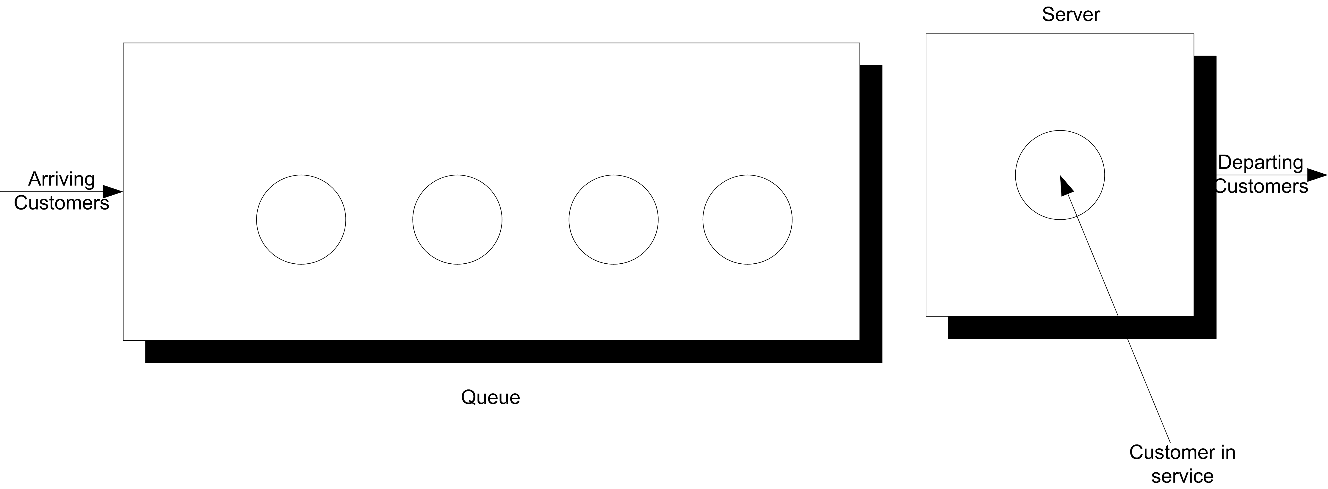
Figure 8.4: Single Server Queueing System
Consider a single server queuing system as illustrated Figure 8.4.
For a single server queueing system, there is an equation that allows the computation of the waiting times of each of the customers based on knowledge of the arrival and service times. Let \(X_1, X_2, \ldots\) represent the successive service times and \(Y_1, Y_2, \ldots\) represent the successive inter-arrival times for each of the customers that visit the queue. Let \(E[Y_i] = 1/\lambda\) be the mean of the inter-arrival times so that \(\lambda\) is the mean arrival rate. Let \(E[Y_i] = 1/\mu\) be the mean of the service times so that \(\mu\) is the mean service rate. Let \(W_i\) be the waiting time in the queue for the \(i^{th}\) customer. That is, the time between when the customer arrives until they enter service.
Lindley’s equation, see (Gross and Harris 1998), relates the waiting time to the arrivals and services as follows:
\[W_{i+1} = max(0, W_i + X_i - Y_i)\]
The relationship says that the time that the \((i + 1)^{st}\) customer must wait is the time the \(i^{th}\) waited, plus the \(i^{th}\) customer’s service time, \(X_i\) (because that customer is in front of the \(i^{th}\) customer), less the time between arrivals of the \(i^{th}\) and \((i + 1)^{st}\) customers, \(Y_i\). If \(W_i + X_i - Y_i\) is less than zero, then the (\((i + 1)^{st}\) customer arrived after the \(i^{th}\) finished service, and thus the waiting time for the \((i + 1)^{st}\) customer is zero, because his service starts immediately.
Suppose that \(X_i \sim exp(E[X_i] = 0.7)\) and \(Y_i \sim exp(E[Y_i] = 1.0)\). This is a M/M/1 queue with \(\lambda\) = 1 and \(\mu\) = 10/7. Thus, based on traditional queuing theory results:
\[\rho = 0.7\]
\[L_q = \dfrac{0.7 \times 0.7}{1 - 0.7} = 1.6\bar{33}\]
\[W_q = \dfrac{L_q}{\lambda} = 1.6\bar{33} \; \text{minutes}\]
Lindley’s equation can be readily implemented in Java as illustrated in the following code listing.
// inter-arrival time distribution
RandomIfc y = new ExponentialRV(1.0);
// service time distribution
RandomIfc x = new ExponentialRV(0.7);
int r = 30; // number of replications
int n = 100000; // number of customers
int d = 10000; // warm up
Statistic avgw = new Statistic("Across rep avg waiting time");
Statistic wbar = new Statistic("Within rep avg waiting time");
for (int i = 1; i <= r; i++) {
    double w = 0; // initial waiting time
    for (int j = 1; j <= n; j++) {
        w = Math.max(0.0, w + x.getValue() - y.getValue());
        wbar.collect(w);// collect waiting time
        if (j == d) {// clear stats at warmup
            wbar.reset();
        }
    }
    //collect across replication statistics
    avgw.collect(wbar.getAverage());
    // clear within replication statistics for next rep
    wbar.reset();
}
System.out.println("Replication/Deletion Lindley Equation Example");
System.out.println(avgw);
This implementation can be readily extended to capture the data to files for display in spreadsheets or other plotting software. As part of the plotting process it is useful to display the cumulative sum and cumulative average of the data values.
\[\sum_{i=1}^n W_i \; \text{for} \; n = 1,2,\ldots\]
\[\dfrac{1}{n} \sum_{i=1}^n W_i \; \text{for} \; n = 1,2,\ldots\]
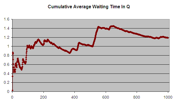
Figure 8.5: Cumulative Average Waiting Time of 1000 Customers
Figure 8.5 presents the cumulative average plot of the first 1000 customers. As seen in the plot, the cumulative average starts out low and then eventually trends towards 1.2 minutes.
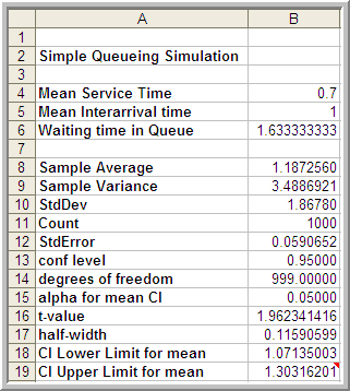
Figure 8.6: Lindley Equation Results Across 1000 Customers
The analytical results indicate that the true long-run expected waiting time in the queue is 1.633 minutes. The average over the 1000 customers in the simulation is 1.187 minutes. The results in Figure 8.6 indicated that the sample average is significantly lower than the true expected average. We will explore why this occurs shortly.
The first issue to consider with this data is independence. To do this you should analyze the 1000 observations in terms of its autocorrelation.
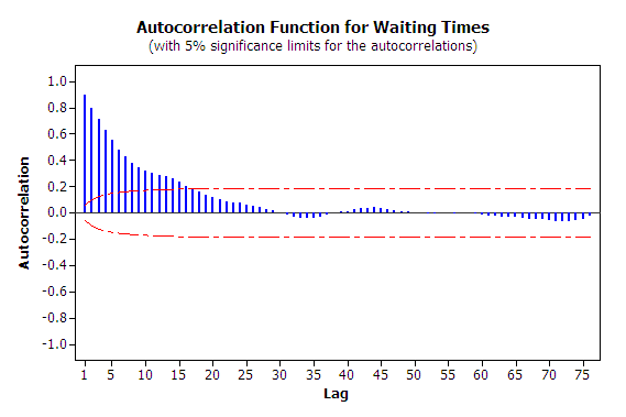
Figure 8.7: Autocorrelation Plot for Waiting Times
From Figure 8.7, it is readily apparent that the data has strong positive correlation. The lag-1 correlation for this data is estimated to be about 0.9. Figure 8.7 clearly indicates the strong first order linear dependence between \(W_i\) and \(W_{i-1}\). This positive dependence implies that if the previous customer waited a long time the next customer is likely to wait a long time. If the previous customer had a short wait, then the next customer is likely to have a short wait. This makes sense with respect to how a queue operates.
Strong positive correlation has serious implications when developing confidence intervals on the mean customer waiting time because the usual estimator for the sample variance:
\[S^2(n) = \dfrac{1}{n - 1} \sum_{i=1}^n (X_i - \bar{X})^2\]
is a biased estimator for the true population variance when there is correlation in the observations. This issue will be re-examined when ways to mitigate these problems are discussed.
The second issue that needs to be discussed is that of the non-stationary behavior of the data. Non-stationary data indicates some dependence on time. More generally, non-stationary implies that the \(W_1, W_2,W_3, \ldots, W_n\) are not obtained from identical distributions.
Why should the distribution of \(W_1\) not be the same as the distribution of \(W_{1000}\)? The first customer is likely to enter the queue with no previous customers present and thus it is very likely that the first customer will experience little or no wait (the way \(W_0\) was initialize in this example allows a chance of waiting for the first customer). However, the \(1000^{th}\) customer may face an entirely different situation. Between the \(1^{st}\) and the \(1000^{th}\) customer there might likely be a line formed. In fact from the M/M/1 formula, it is known that the steady state expected number in the queue is 1.633. Clearly, the conditions that the \(1^{st}\) customer faces are different than the \(1000^{th}\) customer. Thus, the distributions of their waiting times are likely to be different.
This situation can be better understood by considering a model for the underlying data. A time series, \(X_1,X_2,\ldots,\) is said to be covariance stationary if:
The mean exists and \(\theta = E[X_i]\), for i = 1,2,\(\ldots\), n
The variance exists and \(Var[X_i] = \sigma^2\) \(>\) 0, for i = 1,2,\(\ldots\), n
The lag-k autocorrelation, \(\rho_k = cor(X_i, X_{i+k})\), is not a function of i, i.e. the correlation between any two points in the series does not depend upon where the points are in the series, it depends only upon the distance between them in the series.
In the case of the customer waiting times, we can conclude from the discussion that it is very likely that \(\theta \neq E[X_i]\) and \(Var[X_i] \neq \sigma^2\) for each i = 1,2,\(\ldots\), n for the time series.
Do you think that is it likely that the distributions of \(W_{9999}\) and \(W_{10000}\) will be similar? The argument, that the \(9999^{th}\) customer is on average likely to experience similar conditions as the \(10000^{th}\) customer, sure seems reasonable.
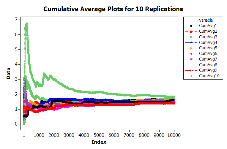
Figure 8.8: Multiple Sample Paths of Queueing Simulation
Figure 8.8 shows 10 different replications of the cumulative average for a 10000 customer simulation. From the figure, we can see that the cumulative average plots can vary significantly over the 10000 customers with the average tracking above the true expected value, below the true expected value, and possibly towards the true expected value. For the case of 10000 customers, you should notice that the cumulative average starts to approach the expected value of the steady state mean waiting time in the queue with increasing number of customers. This is the law of large numbers in action. It appears that it takes a period of time for the performance measure to warm up towards the true mean. Determining the warm up time will be the basic way to mitigate the problem of this non-stationary behavior.
From this discussion, we can conclude that the second basic statistical assumption of identically distributed data is not valid for within replication data. From this, we can also conclude that it is very likely that the data are not normally distributed. In fact, for the M/M/1 it can be shown that the steady state distribution for the waiting time in the queue is not a normal distribution. Thus, all three of the basic statistical assumptions are violated for the within replication data of this example. This problem needs to be addressed in order to properly analyze infinite horizon simulations.
There are two basic methods for performing infinite horizon simulations. The first is to perform multiple replications. This approach addresses independence and normality in a similar fashion as the finite horizon case, but special procedures will be needed to address the non-stationary aspects of the data. The second basic approach is to work with one very long replication. Both of these methods depend on first addressing the problem of the non-stationary aspects of the data. The next section looks at ways to mitigate the non-stationary aspect of within-replication data for infinite horizon simulations.
8.5.1 Assessing the Effect of Initial Conditions
Consider the output stochastic process \(X_i\) of the simulation. Let \(F_i(x|I)\) be the conditional cumulative distribution function of \(X_i\) where \(I\) represents the initial conditions used to start the simulation at time 0. If \(F_i(x|I) \rightarrow F(x)\) when \(i \rightarrow \infty\), for all initial conditions \(I\), then \(F(x)\) is called the steady state distribution of the output process. (Law 2007).
In infinite horizon simulations, estimating parameters of the steady state distribution, \(F(x)\), such as the steady state mean, \(\theta\), is often the key objective. The fundamental difficulty associated with estimating steady state performance is that unless the system is initialized using the steady state distribution (which is not known), there is no way to directly observe the steady state distribution.
It is true that if the steady state distribution exists and you run the simulation long enough the estimators will tend to converge to the desired quantities. Thus, within the infinite horizon simulation context, you must decide on how long to run the simulations and how to handle the effect of the initial conditions on the estimates of performance. The initial conditions of a simulation represent the state of the system when the simulation is started. For example, in simulating the pharmacy system, the simulation was started with no customers in service or in the line. This is referred to as empty and idle. The initial conditions of the simulation affect the rate of convergence of estimators of steady state performance.
Because the distributions \(F_i(x|I)\) at the start of the replication tend to depend more heavily upon the initial conditions, estimators of steady state performance such as the sample average, \(\bar{X}\), will tend to be biased. A point estimator, \(\hat{\theta}\), is an unbiased estimator of the parameter of interest, \(\theta\), if \(E[\hat{\theta}] = \theta\). That is, if the expected value of the sampling distribution is equal to the parameter of interest then the estimator is said to be unbiased. If the estimator is biased then the difference, \(E[\hat{\theta}] - \theta\), is called the bias of, \(\hat{\theta}\), the estimator.
Note that any individual difference between the true parameter, \(\theta\), and a particular observation, \(X_i\), is called error, \(\epsilon_i = X_i -\theta\). If the expected value of the errors is not zero, then there is bias. A particular observation is not biased. Bias is a property of the estimator. Bias is analogous to being consistently off target when shooting at a bulls-eye. It is as if the sights on your gun are crooked. In order to estimate the bias of an estimator, you must have multiple observations of the estimator. Suppose that you are estimating the mean waiting time in the queue as per the previous example and that the estimator is based on the first 20 customers. That is, the estimator is:
\[\bar{W}_r = \dfrac{1}{20}\sum_{i=1}^{20} W_{ir}\]
and there are \(r = 1, 2, \ldots 10\) replications. The following table shows the sample average waiting time for the first 20 customers for 10 different replications.
| r | \(\bar{W}_r\) | \(B_r = \bar{W}_r - W_q\) |
|---|---|---|
| 1 | 0.194114 | -1.43922 |
| 2 | 0.514809 | -1.11852 |
| 3 | 1.127332 | -0.506 |
| 4 | 0.390004 | -1.24333 |
| 5 | 1.05056 | -0.58277 |
| 6 | 1.604883 | -0.02845 |
| 7 | 0.445822 | -1.18751 |
| 8 | 0.610001 | -1.02333 |
| 9 | 0.52462 | -1.10871 |
| 10 | 0.335311 | -1.29802 |
| \(\bar{\bar{W}}\) = 0.6797 | \(\bar{B}\) = -0.9536 |
In the table, \(B_r\) is an estimate of the bias for the \(r^{th}\) replication, where \(W_q = 1.6\bar{33}\). Upon averaging across the replications, it can be seen that \(\bar{B}= -0.9536\), which indicates that the estimator based only on the first 20 customers has significant negative bias, i.e. on average it is less than the target value.
This is the so called initialization bias problem in steady state simulation. Unless the initial conditions of the simulation can be generated according to \(F(x)\), which is not known, you must focus on methods that detect and/or mitigate the presence of initialization bias.
One strategy for initialization bias mitigation is to find an index, \(d\), for the output process, \({X_i}\), so that \({X_i; i = d + 1, \ldots}\) will have substantially similar distributional properties as the steady state distribution \(F(x)\). This is called the simulation warm up problem, where \(d\) is called the warm up point, and \({i = 1,\ldots,d}\) is called the warm up period for the simulation. Then, the estimators of steady state performance are based only on \({X_i; i = d + 1, \ldots}\), which represent the data after deleting the warm up period.
For example, when estimating the steady state mean waiting time for each replication \(r\) the estimator would be:
\[\bar{W_r} = \dfrac{1}{n-d}\sum_{i=d+1}^{n} W_{ir}\]
For time-based performance measures, such as the average number in queue, a time \(T_w\) can be determined past which the data collection process can begin. Estimators of time-persistent performance such as the sample average are computed as:
\[\bar{Y}_r = \dfrac{1}{T_e - T_w}\int_{T_w}^{T_e} Y_r(t) dt\]
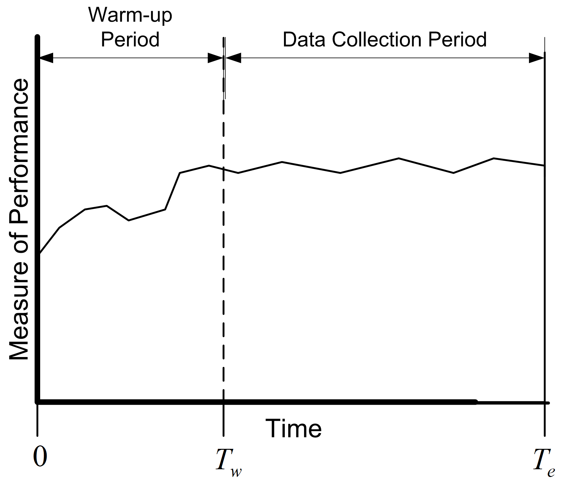
Figure 8.9: The Concept of the Warm Up Period
Figure 8.9 shows the concept of a warm up period for a simulation replication. When you perform a simulation, you can easily specify a time-based warm up period using the setLengthOfWarmUp() method of the Simulation class. In fact, even for observation based data, it will be more convenient to specify the warm up period in terms of time. A given value of \(T_w\) implies a particular value of \(d\) and vice a versa. Specifying a warm up period, causes an event to be scheduled for time \(T_w\). At that time, all the accumulated statistical counters are cleared so that the net effect is that statistics are only collected over the period from \(T_w\) to \(T_e\). The problem then becomes that of finding an appropriate warm up period.
Before proceeding with how to assess the length of the warm up period, the concept of steady state needs to be further examined. This subtle concept is often misunderstood or misrepresented. Often you will hear the phrase: The system has reached steady state. The correct interpretation of this phrase is that the distribution of the desired performance measure has reached a point where it is sufficiently similar to the desired steady state distribution. Steady state is a concept involving the performance measures generated by the system as time goes to infinity. However, sometimes this phrase is interpreted incorrectly to mean that the system itself has reached steady state. Let me state emphatically that the system never reaches steady state. If the system itself reached steady state, then by implication it would never change with respect to time. It should be clear that the system continues to evolve with respect to time; otherwise, it would be a very boring system! Thus, it is incorrect to indicate that the system has reached steady state. Because of this, do not to use the phrase: The system has reached steady state.
Understanding this subtle issue raises an interesting implication concerning the notion of deleting data to remove the initialization bias. Suppose that the state of the system at the end of the warm up period, \(T_w\), is exactly the same as at \(T = 0\). For example, it is certainly possible that at time \(T_w\) for a particular replication that the system was empty and idle. Since the state of the system at \(T_w\) is the same as that of the initial conditions, there will be no effect of deleting the warm up period for this replication. In fact there will be a negative effect, in the sense that data will have been thrown away for no reason. Deletion methods are predicated on the likelihood that the state of the system seen at \(T_w\) is more representative of steady state conditions. At the end of the warm up period, the system can be in any of the possible states of the system. Some states will be more likely than others. If multiple replications are made, then at \(T_w\) each replication will experience a different set of conditions at \(T_w\). Let \(I_{T_w}^r\) be the initial conditions (state) at time \(T_w\) on replication \(r\). By setting a warm up period and performing multiple replications, you are in essence sampling from the distribution governing the state of the system at time \(T_w\). If \(T_w\) is long enough, then on average across the replications, you are more likely to start collecting data when the system is in states that are more representative over the long term (rather than just empty and idle).
Many methods and rules have been proposed to determine the warm up period. The interested reader is referred to (Wilson and Pritsker 1978), Lada, Wilson, and Steiger (2003), (Litton and Harmonosky 2002), White, Cobb, and Spratt (2000), Cash et al. (1992), and (Rossetti and Delaney 1995) for an overview of such methods. This discussion will concentrate on the visual method proposed in (Welch 1983).
The basic idea behind Welch’s graphical procedure is simple:
Make \(R\) replications. Typically, \(R \geq 5\) is recommended.
Let \(Y_{rj}\) be the \(j^{th}\) observation on replication \(r\) for \(j = 1,2,\cdots,m_r\) where \(m_r\) is the number of observations in the \(r^{th}\) replication, and \(r = 1,2,\cdots,n\),
Compute the averages across the replications for each \(j = 1, 2, \ldots, m\), where \(m = min(m_r)\) for \(r = 1,2,\cdots,n\).
\[\bar{Y}_{\cdot j} = \dfrac{1}{n}\sum_{r=1}^n Y_{rj}\]
Plot, \(\bar{Y}_{\cdot j}\) for each \(j = 1, 2, \ldots, m\)
Apply smoothing techniques to \(\bar{Y}_{\cdot j}\) for \(j = 1, 2, \ldots, m\)
Visually assess where the plots start to converge
Let’s apply the Welch’s procedure to the replications generated from the Lindley equation simulation. Using the 10 replications stored in a spreadsheet we can compute the average across each replication for each customer.
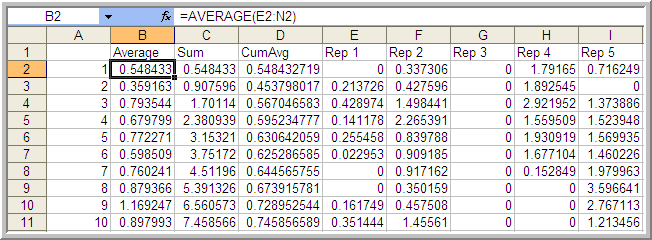
Figure 8.10: Computing the Averages for the Welch Plot
In Figure 8.10, cell B2 represents the average across the 10 replications for the \(1^{st}\) customer. Column D represents the cumulative average associated with column B.
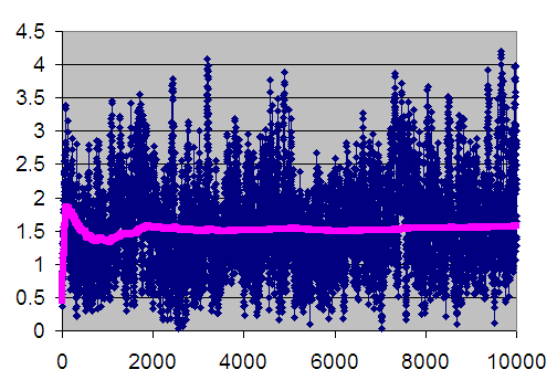
Figure 8.11: Welch Plot with Superimposed Cumulative Average Line
Figure 8.11 is the plot of the cumulative average (column D) superimposed on the averages across replications (column B). The cumulative average is one method of smoothing the data. From the plot, you can infer that after about customer 3000 the cumulative average has started to converge. Thus, from this analysis you might infer that \(d = 3000\).
When you perform an infinite horizon simulation by specifying a warm up period and making multiple replications, you are using the method of replication-deletion. If the method of replication-deletion with \(d = 3000\) is used for the current example, a slight reduction in the bias can be achieved as indicated in the following table.
| \(r\) | \(\bar{W}_r\) \((d = 0)\) | \(\bar{W}_r(d = 3000)\) | \(B_r(d = 0)\) | \(B_r(d = 3000)\) |
|---|---|---|---|---|
| 1 | 1.594843 | 1.592421 | -0.03849 | -0.04091 |
| 2 | 1.452237 | 1.447396 | -0.1811 | -0.18594 |
| 3 | 1.657355 | 1.768249 | 0.024022 | 0.134915 |
| 4 | 1.503747 | 1.443251 | -0.12959 | -0.19008 |
| 5 | 1.606765 | 1.731306 | -0.02657 | 0.097973 |
| 6 | 1.464981 | 1.559769 | -0.16835 | -0.07356 |
| 7 | 1.621275 | 1.75917 | -0.01206 | 0.125837 |
| 8 | 1.600563 | 1.67868 | -0.03277 | 0.045347 |
| 9 | 1.400995 | 1.450852 | -0.23234 | -0.18248 |
| 10 | 1.833414 | 1.604855 | 0.20008 | -0.02848 |
| \(\bar{\bar{W}}\) = 1.573617 | \(\bar{\bar{W}}\) = 1.603595 | \(\bar{B}\) = -0.05972 | \(\bar{B}\) = -0.02974 | |
| s = 0.1248 | s = 0.1286 | s = 0.1248 | s = 0.1286 | |
| 95% LL | 1.4843 | 1.5116 | -0.149023 | -0.121704 |
| 95% UL | 1.6629 | 1.6959 | -0.029590 | 0.062228 |
While not definitive for this simple example, the results suggest that deleting the warm up period helps to reduce initialization bias. This model’s warm up period will be further analyzed using additional tools available in the next section.
In performing the method of replication-deletion, there is a fundamental trade-off that occurs. Because data is deleted, the variability of the estimator will tend to increase while the bias will tend to decrease. This is a trade-off between a reduction in bias and an increase in variance. That is, accuracy is being traded off against precision when deleting the warm up period. In addition to this trade off, data from each replication is also being thrown away. This takes computational time that could be expended more effectively on collecting usable data. Another disadvantage of performing replication-deletion is that the techniques for assessing the warm up period (especially graphical) may require significant data storage. The Welch plotting procedure requires the saving of data points for post processing after the simulation run. In addition, significant time by the analyst may be required to perform the technique and the technique is subjective.
When a simulation has many performance measures, you may have to perform a warm up period analysis for every performance measure. This is particularly important, since in general, the performance measures of the same model may converge towards steady state conditions at different rates. In this case, the length of the warm up period must be sufficiently long enough to cover all the performance measures. Finally, replication-deletion may simply compound the bias problem if the warm up period is insufficient relative to the length of the simulation. If you have not specified a long enough warm up period, you are potentially compounding the problem for \(n\) replications.
Despite all these disadvantages, replication-deletion is very much used in practice because of the simplicity of the analysis after the warm up period has been determined. Once you are satisfied that you have a good warm up period, the analysis of the results is the same as that of finite horizon simulations. Replication-deletion also facilitates the use of experimental design techniques that rely on replicating design points.
The next section illustrates how to perform the method of replication-deletion on this simple M/M/1 model.
8.5.2 Performing the Method of Replication-Deletion
The first step in performing the method of replication-deletion is to determine the length of the warm up period. This example illustrates how to:
Save the values from observation and time-based data to files for post processing
Make Welch plots based on the saved data
Setup and run the multiple replications
Interpret the results
When performing a warm-up period analysis, the first decision to make is the length of each replication. In general, there is very little guidance that can be offered other than to try different run lengths and check for the sensitivity of your results. Within the context of queueing simulations, the work by (Whitt 1989) offers some ideas on specifying the run length, but these results are difficult to translate to general simulations.
Since the purpose here is to determine the length of the warm up period, then the run length should be bigger than what you suspect the warm up period to be. In this analysis, it is better to be conservative. You should make the run length as long as possible given your time and data storage constraints. Banks et al. (2005) offer the rule of thumb that the run length should be at least 10 times the amount of data deleted. That is, \(n \geq 10d\) or in terms of time, \(T_e \geq 10T_w\). Of course, this is a “catch 22” situation because you need to specify \(n\) or equivalently \(T_e\) in order to assess \(T_w\). Setting \(T_e\) very large is recommended when doing a preliminary assessment of \(T_w\). Then, you can use the rule of thumb of 10 times the amount of data deleted when doing a more serious assessment of \(T_w\) (e.g. using Welch plots etc.)
A preliminary assessment of the current model has already been performed based on the previously described spreadsheet simulation. That assessment suggested a deletion point of at least \(d = 3000\) customers. This can be used as a starting point in the current effort. Now, \(T_w\) needs to be determined based on \(d\). The value of \(d\) represents the customer number for the end of the warm up period. To get \(T_w\), you need to answer the question: How long (on average) will it take for the simulation to generate \(d\) observations. In this model, the mean number of arrivals is 1 customer per minute. Thus, the initial \(T_w\) is
\[3000 \; \text{customers} \times \frac{\text{minute}}{\text{1 customer}} \; = 3000 \; \text{minutes}\]
and therefore the initial \(T_e\) should be 30,000 minutes. That is, you should specify 30,000 minutes for the replication length.
8.5.2.1 Determining the Warm Up Period
To perform a more rigorous analysis of the warm up period, we need to run the simulation for multiple replications and capture the data necessary to produce Welch plots for the performance measures of interest. Within the JSL, this can be accomplished by using the classes within the welch package in the JSL utilities. There are three classes of note:
WelchDataFileCollectorThis class captures data associated with a ResponseVariable within the simulation model. Every observation from every replication is written to a binary data file. In addition, a text based data file is created that contains the meta data associated with the data collection process. The meta data file records the number of replications, the number of observations for each replication, and the time between observations for each replication.
WelchDataFileCollectorTWThis class has the same functionality as the WelchDataFileCollector class except for TimeWeighted response variables. In this case, a discretizing interval must be provided in order to batch the time weighted observations into discrete intervals.
WelchDataFileAnalyzerThis class uses the files produced by the previous two classes to produces the Welch data. That is, the average across each row of observations and the cumulative average over the observations. This class produces files from which the plots can be made.
A warm up period analysis is associated with a particular response. The goal is to determine the number of observations of the response to delete at the beginning of the simulation. We can collect the relevant data by attaching an observer to the response variable. In the following listing, lines 8 and 9 get access to the two responses from the model. Then, in lines 12-16, the data collectors are created and attached to the responses. This needs to be done before the simulation is executed. The simulation is then run and then, the WelchDataFileAnalyzer instances for each of the responses are made. The Welch plot data is written to a file for plotting. Finally, the Welch chart is displayed. This code illustrates the display for the system time. In a similar manner the Welch plot for the number in the system can be performed.
Simulation sim = new Simulation("DTP");
// get the model
Model m = sim.getModel();
// add DriveThroughPharmacy to the main model
DriveThroughPharmacy driveThroughPharmacy = new DriveThroughPharmacy(m);
driveThroughPharmacy.setArrivalRS(new ExponentialRV(1.0));
driveThroughPharmacy.setServiceRS(new ExponentialRV(0.7));
ResponseVariable rv = m.getResponseVariable("System Time");
TimeWeighted tw = m.getTimeWeighted("# in System");
File d = JSL.makeOutputSubDirectory(sim.getName());
// this creates files to capture welch data from a ResponseVariable
WelchDataFileCollector wdfc = new WelchDataFileCollector(d, "welchsystime");
rv.addObserver(wdfc);
// this creates files to collection welch data from a TimeWeighted variable
WelchDataFileCollectorTW wdfctw = new WelchDataFileCollectorTW(10, d, "numInSystem");
tw.addObserver(wdfctw);
// set the parameters of the experiment
sim.setNumberOfReplications(5);
sim.setLengthOfReplication(5000.0);
SimulationReporter r = sim.makeSimulationReporter();
System.out.println("Simulation started.");
sim.run();
System.out.println("Simulation completed.");
r.printAcrossReplicationSummaryStatistics();
System.out.println(wdfc);
WelchDataFileAnalyzer wa = wdfc.makeWelchDataFileAnalyzer();
System.out.println(wa);

System.out.println("Writing welch data to csv");
wa.makeCSVWelchPlotDataFile();
System.out.println("Writing welch data to welch data file");
wa.makeWelchPlotDataFile();
System.out.println("Plotting the Welch plot for System Times");
WelchChart.display(wa);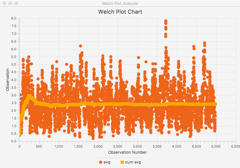
Figure 8.12: Welch Plot for System Time Analysis
Figure 8.12 illustrates the plot of the data. From this plot, we can estimate the number of observations to delete as 2000.
Time-persistent observations are saved within a file from within the model such that the time of the observation and the value of the state variable at the time of change are recorded. Thus, the observations are not equally spaced in time. In order to perform the Welch plot analysis, we need to cut the data into discrete equally spaced intervals of time.
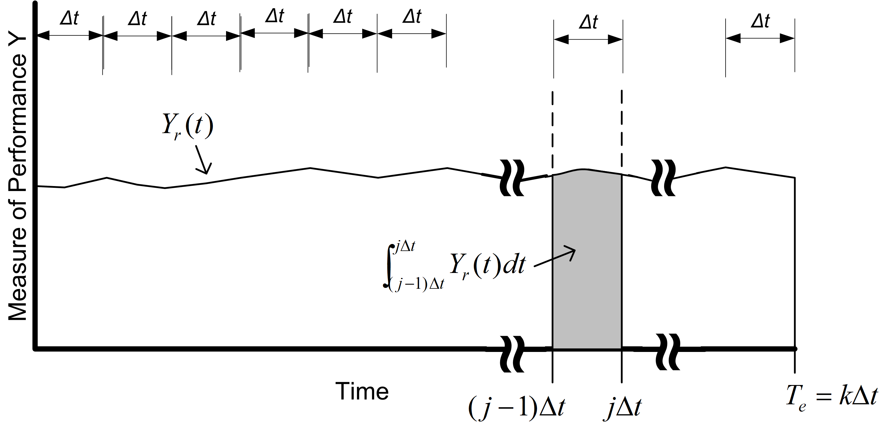
Figure 8.13: Discretizing Time-Persistent Data
Figure 8.13 illustrates the concept of discretizing time-persistent data. Suppose that you divide \(T_e\) into \(k\) intervals of size \(\Delta t\), so that \(T_e = k \times \Delta t\). The time average over the \(j^{th}\) interval is given by:
\[\bar{Y}_{rj} = \dfrac{1}{\Delta t} \int_{j-1) \Delta t}^{j \Delta t} Y_r(t)dt\]
Thus, the overall time average can be computed from the time average associated with each interval:
\[\begin{aligned} \bar{Y}_{r} & = \dfrac{\int_0^{T_e} Y_r (t)dt}{T_e} =\dfrac{\int_0^{T_e} Y_r (t)dt}{k \Delta t} \\ & = \dfrac{\sum_{j=1}^{k}\int_{(j-1) \Delta t}^{j \Delta t} Y_r (t)dt}{k \Delta t} = \dfrac{\sum_{j=1}^{k} \bar{Y}_{rj}}{k}\end{aligned}\]
Each of the \(\bar{Y}_{rj}\) are computed over intervals of time that are equally spaced and can be treated as if they are observation (tally) based data.
The computation of the \(\bar{Y}_{rj}\) for time-persistent data can be achieved by using the WelchDataFileCollectorTW class and specifying a discretization interval. Since the number in queue data is time-persistent, time based batches are selected, and the batch size is specified in terms of time. In this case, the data is being batched based on a time interval of 10 minutes in line 15 of the code listing. This produces a file which contains the \(\bar{Y}_{rj}\) as observations. This file can then be analyzed as previously illustrated.
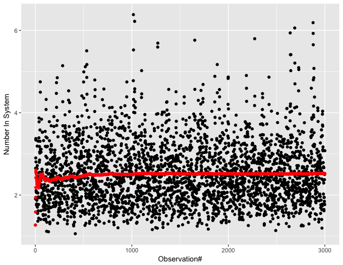
Figure 8.14: Welch Plot of Time-Persistent Number in System Data
The resulting plot is show in Figure 8.14. This plot is sparser than the previous plot because each observation represents the average of 10 minutes. There are 3000 observations. From the plot, we can conclude that after observation 1000, we see a steady convergence. The 1000th observation represents 10000 time units (minutes) because every observation represents 10 time units.
Once you have performed the warm up analysis, you still need to use your simulation model to estimate system performance. Because the process of analyzing the warm up period involves saving the data you could use the already saved data to estimate your system performance after truncating the initial portion of the data from the data sets. If re-running the simulation is relatively inexpensive, then you can simply set the warm up period via the Simulation class and re-run the model. Following the rule of thumb that the length of the run should be at least 10 times the warm up period, the simulation was re-run with the settings (30 replications, 10000 minute warm up period, 100,000 minute replication length). The results shown in the following table indicate that there does not appear to be any significant bias with these replication settings.
| Response Name | \(\bar{x}\) | \(s\) |
|---|---|---|
| PharmacyQ:Num In Q | 1.637069 | 0.040491 |
| PharmacyQ:Time In Q | 1.636834 | 0.037817 |
| NumBusy | 0.700038 | 0.003435 |
| Number in System | 2.337107 | 0.043385 |
| System Time | 2.336790 | 0.039586 |
| Number of Replications | 30 |
The true waiting time in the queue is \(1.6\bar{33}\) and it is clear that the 95% confidence interval contains this value.
The process described here for determining the warm up period for steady state simulation is tedious and time consuming. Research into automating this process is still an active area of investigation. The recent work by (Robinson 2005) and Rossetti and Li (2005) holds some promise in this regard; however, there remains the need to integrate these methods into computer simulation software. Even though determining the warm up period is tedious, some consideration of the warm up period should be done for infinite horizon simulations.
Once the warm up period has been found, you can set the warm up period using the Simulation class. Then, you can use the method of replication-deletion to perform your simulation experiments. Thus, all the discussion previously presented on the analysis of finite horizon simulations can be applied.
When determining the number of replications, you can apply the fixed sample size procedure after performing a pilot run. If the analysis indicates that you need to make more runs to meet your confidence interval half-width you have two alternatives: 1) increase the number of replications or 2) keep the same number of replications but increase the length of each replication. If \(n_0\) was the initial number of replications and \(n\) is the number of replications recommended by the sample size determination procedure, then you can instead set \(T_e\) equal to \((n/n_0)T_e\) and run \(n_0\) replications. Thus, you will still have approximately the same amount of data collected over your replications, but the longer run length may reduce the effect of initialization bias.
As previously mentioned, the method of replication-deletion causes each replication to delete the initial portion of the run. As an alternative, you can make one long run and delete the initial portion only once. When analyzing an infinite horizon simulation based on one long replication, a method is needed to address the correlation present in the within replication data. The method of batch means is often used in this case and has been automated in within the JSL. The next section discusses the statistical basis for the batch means method and addresses some of the practical issues of using it within the JSL.
8.5.3 The Method of Batch Means
In the batch mean method, only one simulation run is executed. After deleting the warm up period, the remainder of the run is divided into \(k\) batches, with each batch average representing a single observation.
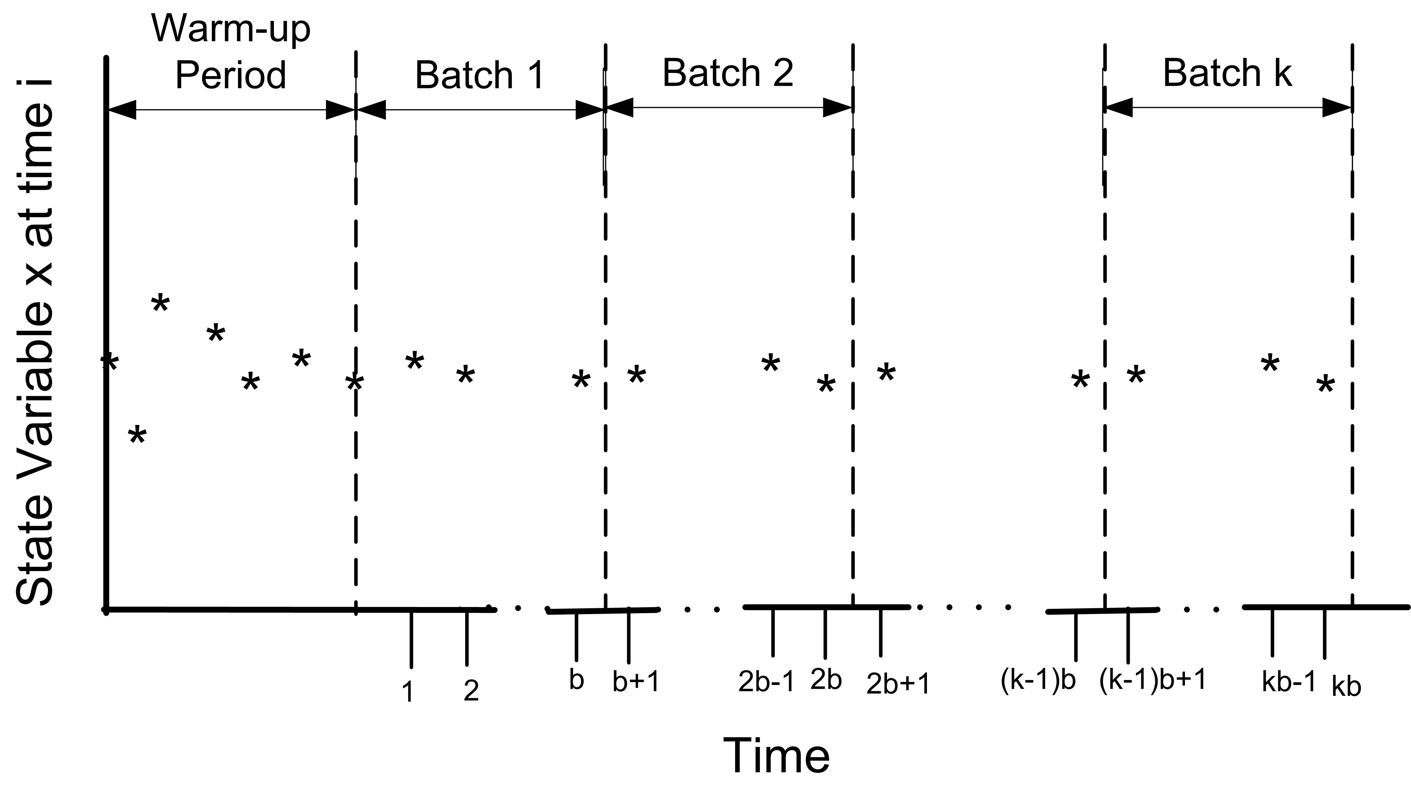
Figure 8.15: Illustration of the Batch MeansMethod
Figure 8.15 illustrates the concept of batching observations. The advantages of the batch means method are that it entails a long simulation run, thus dampening the effect of the initial conditions. The disadvantage is that the within replication data are correlated and unless properly formed the batches may also exhibit a strong degree of correlation.
The following presentation assumes that a warm up analysis has already been performed and that the data that has been collected occurs after the warm up period. For simplicity, the presentation assumes observation based data. The discussion also applies to time-based data that has been cut into discrete equally spaced intervals of time as previously described. Therefore, assume that a series of observations, \((X_1, X_2, X_3, \ldots, X_n)\), is available from within the one long replication after the warm up period. As shown earlier, the within replication data can be highly correlated. In that section, it was mentioned that standard confidence intervals based on
\[S^2(n) = \dfrac{1}{n - 1}\sum_{i=1}^n (X_i - \bar{X})^2\]
are not appropriate for this type of data. Suppose you were to ignore the correlation, what would be the harm? In essence, a confidence interval implies a certain level of confidence in the decisions based on the confidence interval. When you use \(S^2(n)\) as defined above, you will not achieve the desired level of confidence because \(S^2(n)\) is a biased estimator for the variance of \(\bar{X}\) when the data are correlated. Under the assumption that the data are covariance stationary, an assessment of the harm in ignoring the correlation can be made. For a series that is covariance stationary, one can show that
\[Var(\bar{X}) = \dfrac{\gamma_0}{n} \left[1 + 2 \sum_{k=1}^{n-1} \left(1 - \dfrac{k}{n} \right) \rho_k \right]\]
where \(\gamma_0 = Var(X_i)\), \(\gamma_k = Cov(X_i, X_{i + k})\), and \(\rho_k = \gamma_k/\gamma_0\) for \(k = 1, 2, \ldots, n - 1\).
When the data are correlated, \(S^2/n\) is a biased estimator of \(Var(\bar{X})\). To show this, you need to compute the expected value of \(S^2/n\) as follows:
\[E\left[S^2/n\right] = \dfrac{\gamma_0}{n} \left[1 - \dfrac{2R}{n - 1}\right]\]
where
\[R = \sum_{k=1}^{n-1} (1 - \dfrac{k}{n}) \rho_k\]
Bias is defined as the difference between the expected value of the estimator and the quantity being estimated. In this case, the bias can be computed with some algebra as:
\[\text{Bias} = E\left[S^2/n\right] - Var(\bar{Y}) = \dfrac{-2 \gamma_0 R}{n - 1}\]
Since \(\gamma_0 > 0\) and \(n > 1\) the sign of the bias depends on the quantity R and thus on the correlation. There are three cases to consider: zero correlation, negative correlation, and positive correlation. Since \(-1 \leq \rho_k \leq 1\), examining the limiting values for the correlation will determine the range of the bias.
For positive correlation, \(0 \leq \rho_k \leq 1\), the bias will be negative, (\(- \gamma_0 \leq Bias \leq 0\)). Thus, the bias is negative if the correlation is positive, and the bias is positive if the correlation is negative. In the case of positive correlation, \(S^2/n\) underestimates the \(Var(\bar{X})\). Thus, using \(S^2/n\) to form confidence intervals will make the confidence intervals too short. You will have unjustified confidence in the point estimate in this case. The true confidence will not be the desired \(1 - \alpha\). Decisions based on positively correlated data will have a higher than planned risk of making an error based on the confidence interval.
One can easily show that for negative correlation, \(-1 \leq \rho_k \leq 0\), the bias will be positive (\(0 \leq Bias \leq \gamma_0\)). In the case of negatively correlated data, \(S^2/n\) over estimates the \(Var(\bar{X})\). A confidence interval based on \(S^2/n\) will be too wide and the true quality of the estimate will be better than indicated. The true confidence coefficient will not be the desired \(1 - \alpha\); it will be greater than \(1 - \alpha\).
Of the two cases, the positively correlated case is the more severe in terms of its effect on the decision making process; however, both are problems. Thus, the naive use of \(S^2/n\) for dependent data is highly unwarranted. If you want to build confidence intervals on \(\bar{X}\) you need to find an unbiased estimator of the \(Var(\bar{X})\).
The method of batch means provides a way to develop (at least approximately) an unbiased estimator for \(Var(\bar{X})\). Assuming that you have a series of data point, the method of batch means method divides the data into subsequences of contiguous batches:
\[\begin{gathered} \underbrace{X_1, X_2, \ldots, X_b}_{batch 1} \cdots \underbrace{X_{b+1}, X_{b+2}, \ldots, X_{2b}}_{batch 2} \cdots \\ \underbrace{X_{(j-1)b+1}, X_{(j-1)b+2}, \ldots, X_{jb}}_{batch j} \cdots \underbrace{X_{(k-1)b+1}, X_{(k-1)b+2}, \ldots, X_{kb}}_{batch k}\end{gathered}\]
and computes the sample average of the batches. Let \(k\) be the number of batches each consisting of \(b\) observations, so that \(k = \lfloor n/b \rfloor\). If \(b\) is not a divisor of \(n\) then the last \((n - kb)\) data points will not be used. Define \(\bar{X}_j(b)\) as the \(j^{th}\) batch mean for \(j = 1, 2, \ldots, k\), where,
\[\bar{X}_j(b) = \dfrac{1}{b} \sum_{i=1}^b X_{(j-1)b+i}\]
Each of the batch means are treated like observations in the batch means series. For example, if the batch means are re-labeled as \(Y_j = \bar{X}_j(b)\), the batching process simply produces another series of data, (\(Y_1, Y_2, Y_3, \ldots, Y_k\)) which may be more like a random sample. To form a \(1 - \alpha\)% confidence interval, you simply treat this new series like a random sample and compute approximate confidence intervals using the sample average and sample variance of the batch means series:
\[\bar{Y}(k) = \dfrac{1}{k} \sum_{j=1}^k Y_j\]
\[S_b^2 (k) = \dfrac{1}{k - 1} \sum_{j=1}^k (Y_j - \bar{Y}^2)\]
\[\bar{Y}(k) \pm t_{\alpha/2, k-1} \dfrac{S_b (k)}{\sqrt{k}}\]
Since the original X’s are covariance stationary, it follows that the resulting batch means are also covariance stationary. One can show, see (Alexopoulos and Seila 1998), that the correlation in the batch means reduces as both the size of the batches, \(b\) and the number of data points, \(n\) increases. In addition, one can show that \(S_b^2 (k)/k\) approximates \(\text{Var}(\bar{X})\) with error that reduces as both \(b\) and \(n\) increase towards infinity.
The basic difficulty with the batch means method is determining the batch size or alternatively the number of batches. Larger batch sizes are good for independence but reduce the number of batches, resulting in higher variance for the estimator. (Schmeiser 1982) performed an analysis that suggests that there is little benefit if the number of batches is larger than 30 and recommended that the number of batches remain in the range from 10 to 30. However, when trying to access whether or not the batches are independent it is better to have a large number of batches (\(>\) 100) so that tests on the lag-k correlation have better statistical properties.
There are a variety of procedures that have been developed that will automatically batch the data as it is collected, see for example (Fishman and Yarberry 1997), (Steiger and Wilson 2002), and Banks et al. (2005). has its own batching algorithm. The batching algorithm is described in Kelton, Sadowski, and Sturrock (2004) page 311. See also (Fishman 2001) page 254 for an analysis of the effectiveness of the algorithm.
The discussion here is based on the description in Kelton, Sadowski, and Sturrock (2004). When the algorithm has recorded a sufficient amount of data, it begins by forming k = 20 batches. As more data is collected, additional batches are formed until k = 40 batches are collected. When 40 batches are formed, the algorithm collapses the number of batches back to 20, by averaging each pair of batches. This has the net effect of doubling the batch size. This process is repeated as more data is collected, thereby ensuring that the number of batches is between 20 and 39.
For time-persistent data, the approach requires that the data be discretized as previously discussed in the section on warm up period analysis. Then, the same batch method is applied to ensure between 20 and 39 batches. In addition, the process also computes the lag-1 correlation so that a test can be performed to check if the correlation is significant by testing the hypothesis that the batch means are uncorrelated using the following test statistic, see (Alexopoulos and Seila 1998):
\[C = \sqrt{\dfrac{k^2 - 1}{k - 2}}\biggl[ \hat{\rho}_1 + \dfrac{[Y_1 - \bar{Y}]^2 + [Y_k - \bar{Y}]^2}{2 \sum_{j=1}^k (Y_j - \bar{Y})^2}\biggr]\]
\[\hat{\rho}_1 = \dfrac{\sum_{j=1}^{k-1} (Y_j - \bar{Y})(Y_{j+1} - \bar{Y})}{\sum _{j=1}^k (Y_j - \bar{Y})^2}\]
The hypothesis is rejected if \(C > z_\alpha\) for a given confidence level \(\alpha\). If the batch means do not pass the test, Correlated is reported for the half-width on the statistical reports.
8.5.4 Performing the Method of Batch Means
Performing the method of batch means in the JSL is relatively straight forward. The following assumes that a warm up period analysis has already been performed. Batches are formed during the simulation run and the confidence intervals are based on the batches. In this situation, the primary concern will be to determine the run length that will ensure a desired half-width on the confidence intervals. Both fixed sampling and sequential sampling methods can be applied.
The following code present the process to set up batching
within the JSL for the Drive Through Pharmacy Model. The key class is
the StatisticalBatchingElement class, which must be added to the Model
(see line 9) prior to running the simulation. Then, starting at line 20
the batch summary statistical reporting is captured. The
StatisticalBatchingElement has one key parameter which represents the
interval used to discretize the time weighted variables. If no interval
is supplied, then the algorithm ensures that the initial number of
batches collected before applying the previously described batching
algorithm is 512.
Simulation sim = new Simulation("Drive Through Pharmacy");
Model m = sim.getModel();
// add DriveThroughPharmacy to the main model
DriveThroughPharmacy driveThroughPharmacy = new DriveThroughPharmacy(m);
driveThroughPharmacy.setArrivalRS(new ExponentialRV(1.0));
driveThroughPharmacy.setServiceRS(new ExponentialRV(0.7));

// create the batching element for the simulation
StatisticalBatchingElement be = new StatisticalBatchingElement(m);

// set the parameters of the experiment
sim.setNumberOfReplications(1);
sim.setLengthOfReplication(1300000.0);
sim.setLengthOfWarmUp(100000.0);
System.out.println("Simulation started.");
sim.run();
System.out.println("Simulation completed.");

// get a StatisticReport from the batching element
StatisticReporter statisticReporter = be.getStatisticReporter();

// print out the report
System.out.println(statisticReporter.getHalfWidthSummaryReport());
//System.out.println(be.asString());

// use the name of a response to get a reference to a particular response variable
ResponseVariable systemTime = m.getResponseVariable("System Time");
// access the batch statistic from the batching element
BatchStatistic batchStatistic = be.getBatchStatistic(systemTime);
// get the actual batch mean values
double[] batchMeanArrayCopy = batchStatistic.getBatchMeanArrayCopy();
System.out.println(Arrays.toString(batchMeanArrayCopy));
The analysis performed to determine the warm up period should give you some information concerning how long to make this single run and how long to set it’s warm up period. Assume that a warm up analysis has been performed using \(n_0\) replications of length \(T_e\) and that the analysis has indicated a warm up period of length \(T_w\). Then, we can use this information is setting up the run length and warm up period for the single replication experiment.
As previously discussed, the method of replication deletion spreads the risk of choosing a bad initial condition across multiple replications. The method of batch means relies on only one replication. If you were satisfied with the warm up period analysis based on \(n_0\) replications and you were going to perform replication deletion, then you are willing to throw away the observations contained in at least \(n_0 \times T_w\) time units and you are willing to use the data collected over \(n_0 \times (T_e - T_w)\) time units. Therefore, the warm up period for the single replication can be set at \(n_0 \times T_w\) and the run length can be set at \(n_0 \times T_e\). For example, suppose your warm up analysis was based on the initial results of \(n_0\) = 10, \(T_e\) = 30000, \(T_w\) = 10000. Thus, your starting run length would be \(n_0 \times T_e = 10 \times 30,000 = 300,000\) and the warm period will be \(n_0 \times T_w = 100,000\). The following table show the results based on replication deletion
| Response Name | \(n\) | \(\bar{x}\) | \(hw\) |
|---|---|---|---|
| PharmacyQ:Num In Q | 10 | 1.656893 | 0.084475 |
| PharmacyQ:Time In Q | 10 | 1.659100 | 0.082517 |
| NumBusy | 10 | 0.699705 | 0.004851 |
| Num in System | 10 | 2.356598 | 0.088234 |
| System Time | 10 | 2.359899 | 0.085361 |
This table shows the results based on batching one long replication.
| Response Name | \(n\) | \(\bar{x}\) | \(hw\) |
|---|---|---|---|
| PharmacyQ:Num In Q | 32 | 1.631132 | 0.047416 |
| PharmacyQ:Time In Q | 24 | 1.627059 | 0.055888 |
| NumBusy | 32 | 0.699278 | 0.004185 |
| Num in System | 32 | 2.330410 | 0.049853 |
| System Time | 24 | 2.324590 | 0.057446 |
Suppose now you want to ensure that the half-widths from a single replication are less than a given error bound. The half-widths reported by the simulation for a single replication are based on the batch means. You can get an approximate idea of how much to increase the length of the replication by using the half-width sample size determination formula.
\[n \cong n_0 \left(\dfrac{h_0}{h}\right)^2\]
In this case, you interpret \(n\) and \(n_0\) as the number of batches. From previous results, there were 32 batches for the time-weighted variables. Based on \(T_e = 300000\) and \(T_w = 100000\) there was a total of \(T_e - T_w = 200000\) time units of observed data. This means that each batch represents \(200,000\div 32 = 6250\) time units. Using this information in the half-width based sample size formula with \(n_0 = 32\), \(h_0 = 0.049\), and \(h = 0.02\), for the number in the system, yields:
\[n \cong n_0 \dfrac{h_0^2}{h^2} = 32 \times \dfrac{(0.049)^2}{(0.02)^2} = 192 \ \ \text{batches}\]
Since each batch in the run had 6250 time units, this yields the need for 1,200,000 time units of observations. Because of the warm up period, you therefore need to set \(T_e\) equal to (1,200,000 + 100,000 = 1,300,000). Re-running the simulation yields the results shown in the following table. The results show that the half-width meets the desired criteria. This approach is approximate since you do not know how the observations will be batched when making the final run.
| Response Name | \(n\) | \(\bar{x}\) | \(hw\) |
|---|---|---|---|
| NumBusy | 32 | 0.698973 | 0.001652 |
| Num in System | 32 | 2.322050 | 0.019413 |
| PharmacyQ:Num In Q | 32 | 1.623077 | 0.018586 |
| PharmacyQ:Time In Q | 36 | 1.625395 | 0.017383 |
| System Time | 36 | 2.324915 | 0.017815 |
Rather than trying to fix the amount of sampling, you might instead try to use a sequential sampling technique that is based on the half-width computed during the simulation run. In order to do this, we need to create a specific observer that can stop the simulation when the half-width criteria is met. Currently, the JSL does not facilitate this approach.
Once the warm up period has been analyzed, performing infinite horizon simulations using the batch means method is relatively straight forward. A disadvantage of the batch means method is that it will be more difficult to use the statistical classical experimental design methods. If you are faced with an infinite horizon simulation, then you can use either the replication-deletion approach or the batch means method readily within the JSL. In either case, you should investigate if there may be any problems related to initialization bias. If you use the replication-deletion approach, you should play it safe when specifying the warm up period. Making the warm up period longer than you think it should be is better than replicating a poor choice. When performing an infinite horizon simulation based on one long run, you should make sure that your run length is long enough. A long run length can help to “wash out” the effects of initial condition bias.
Ideally, in the situation where you have to make many simulation experiments using different parameter settings of the same model, you should perform a warm up analysis for each design configuration. In practice, this is not readily feasible when there are a large number of experiments. In this situation, you should use your common sense to pick the design configurations (and performance measures) that you feel will most likely suffer from initialization bias. If you can determine long enough warm up periods for these configurations, the other configurations should be relatively safe from the problem by using the longest warm up period found.
There are a number of other techniques that have been developed for the analysis of infinite horizon simulations including the standardized time series method, the regenerative method, and spectral methods. An overview of these methods and others can be found in (Alexopoulos and Seila 1998) and in (Law 2007).
So far you have learned how to analyze the data from one design configuration. A key use of simulation is to be able to compare alternative system configurations and to assist in choosing which configurations are best according to the decision criteria. The next section discusses how to compare different system configurations.