3.1 Collecting Statistics
The KSL has a wide variety of classes that support statistic computations. A main theme in understanding the usage of the classes within the ksl.utilities.statistics package is the concept of collection. This concept is encapsulated within the CollectorIfc interface. The methods of the CollectorIfc interface are illustrated in Figure 3.1.
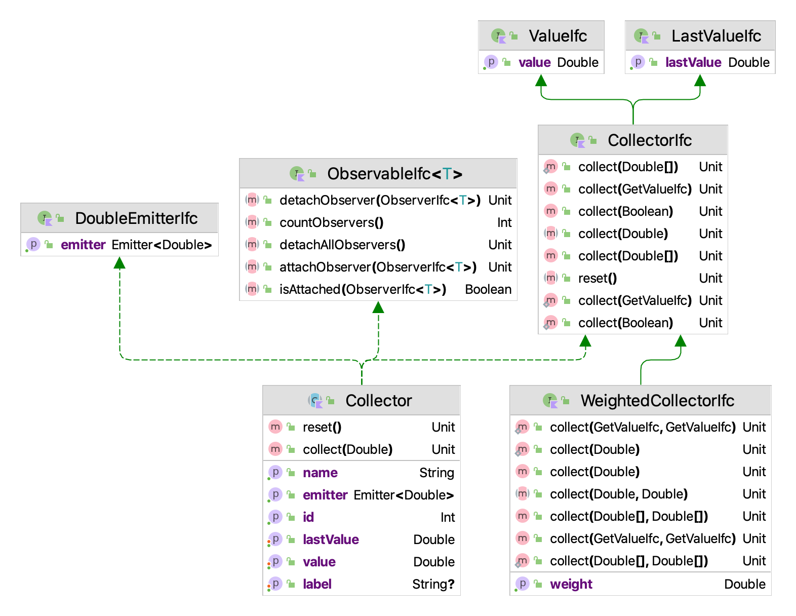
Figure 3.1: CollectorIfc Interface
Something is a collector, if it implements the CollectorIfc interface. The implication is that those values presented to the various collect methods will be observed and tabulated into various quantities based on the presented values. The collect method has been overloaded to facilitate collection of double values, arrays of double values, and boolean values. A collector can be reset. Resetting a collector should set the state of the collector as if no values had been observed. Thus, resetting a collector should clear all previous collection results. The collector may or may not store any of the observations related to the collection process. By default, the standard approach taken is not to store the observations, but rather to summarize the observations in some manner. To facilitate the further use of the observed values, the base class, Collector is observable and will also emit observed values. Thus, other classes can be connected to a base observation process.
Figure 3.2 presents the major classes and interfaces within the statistics package. The CollectIfc interface is implemented within the abstract base class Collector, which serves as the basis for various concrete implementations of statistical collectors. There are two major kinds of statistics, one of which assumes that the values presented must be weighted, the WeightedStatisticIfc interface and the WeightedStatistic class. The other branch of classes, derived from AbstractStatistic do not necessarily have to be weighted. The main classes to be discussed in this chapter are Statistic and Histogram.
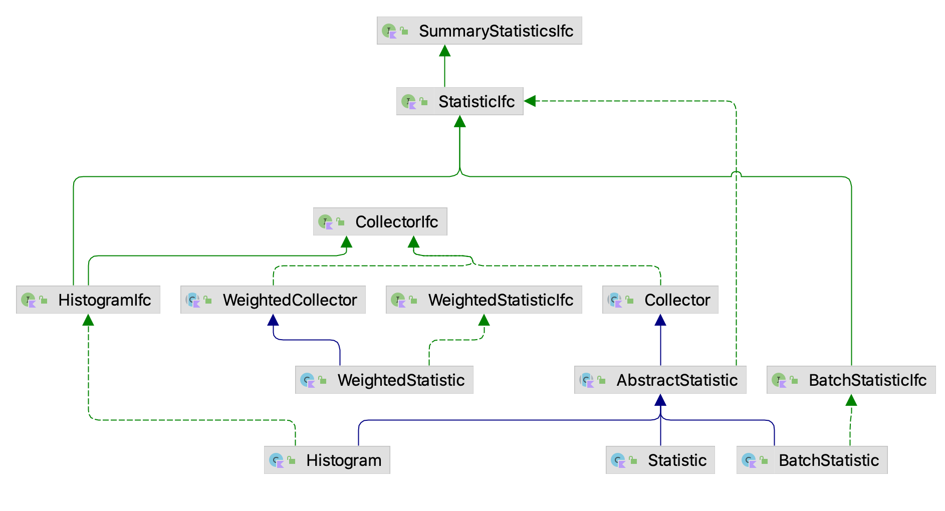
Figure 3.2: Major Classes and Interfaces in the Statistics Package
3.1.1 Creating and Using a Statistic
The Statistic class has a great deal of functionality. It accumulates summary statistics on the values presented to it via its collect methods. Recall also that since the Statistic class implements the CollectorIfc interface, you can use the reset() method to clear all accumulated statistics and reuse the Statistic instance. The major statistical quantities are found in the StatisticIfc interface.
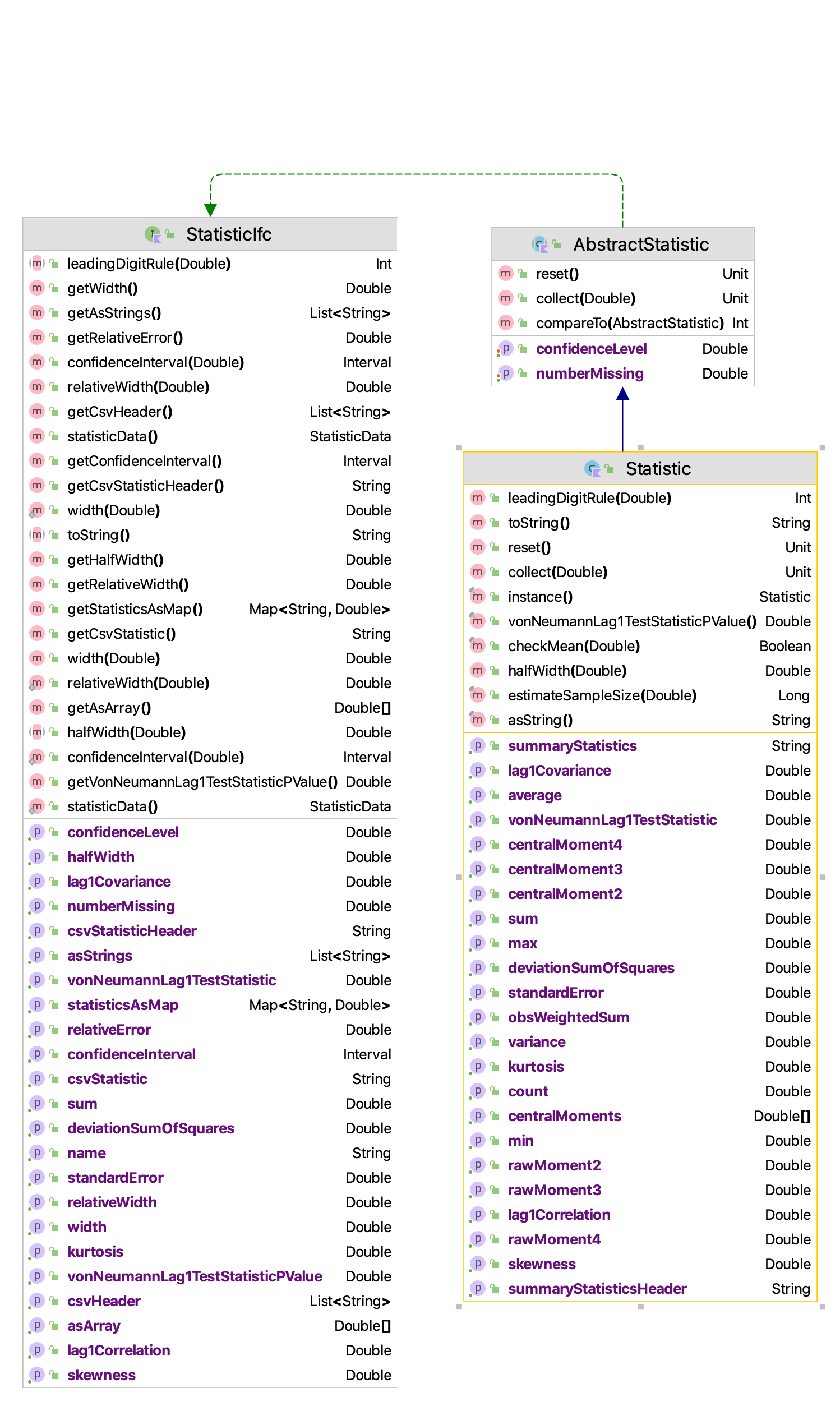
Figure 3.3: Major Accumulated Statistical Quantities
As can be seen in Figure 3.3, the Statistic class not only computes the standard statistical quantities such as the count, average, and variance, it also has functionality to compute confidence intervals, skewness, kurtosis, the minimum, the maximum, and lag 1 covariance and correlation. The computed confidence intervals are based on the assumption that the observed data are normally distributed or that the sample size is large enough to justify using the central limit theorem to assume that the sampling distribution is normal. Thus, we can assume that the confidence intervals are approximate. The summary statistics are computed via efficient one pass algorithms that do not require any observed data to be stored. The algorithms are designed to minimize issues related to numerical precision within the calculated results. The toString() method of the Statistic class has been overridden to contain all of the computed values. Let’s illustrate the usage of the Statistic class with some code. In this code, first we create a normal random variable to be able to generate some data. Then, two statistics are created. The first statistic directly collects the generated values. The second statistic is designed to collect \(P(X\geq 20.0)\) by observing whether the generated value meets this criteria as defined by the boolean expression x >= 20.0.
Example 3.1 (Creating and Using Statistics) This example illustrates how to create instances of the Statistic class to collect randomly generated observations from a normal distribution.
fun main() {
    // create a normal mean = 20.0, variance = 4.0 random variable
    val n = NormalRV(20.0, 4.0, streamNum = 3)
    // create a Statistic to observe the values
    val stat = Statistic("Normal Stats")
    val pGT20 = Statistic("P(X>=20")
    // generate 100 values
    for (i in 1..100) {
        // getValue() method returns generated values
        val x = n.value
        stat.collect(x)
        pGT20.collect(x >= 20.0)
    }
    println(stat)
    println(pGT20)
    val reporter = StatisticReporter(mutableListOf(stat, pGT20))
    println(reporter.halfWidthSummaryReport())
}
The results for the statistics collected directly on the observations from the toString() method are as follows.
ID 1
Name Normal Stats
Number 100.0
Average 20.370190128861807
Standard Deviation 2.111292233346322
Standard Error 0.2111292233346322
Half-width 0.4189261806189412
Confidence Level 0.95
Confidence Interval [19.951263948242865, 20.78911630948075]
Minimum 15.020744984423821
Maximum 25.33588436770212
Sum 2037.0190128861807
Variance 4.457554894588499
Weighted Average 20.370190128861797
Weighted Sum 2037.0190128861796
Sum of Weights 100.0
Weighted Sum of Squares 41935.76252316213
Deviation Sum of Squares 441.2979345642614
Last value collected 21.110736402119805
Last weighted collected 1.0
Kurtosis -0.534855387072145
Skewness 0.20030433873223502
Lag 1 Covariance -0.973414579833684
Lag 1 Correlation -0.22057990840016864
Von Neumann Lag 1 Test Statistic -2.2136062395518343
Number of missing observations 0.0
Lead-Digit Rule(1) -1
Of course, this is probably more output than what you need, but you can use the properties and methods illustrated in Figure 3.3 to access specific desired quantities.
Notice that in the code example that the \(P(X \geq 20.0)\) is also collected. This is done by using the boolean expression x >= 20.0 within the collect() method. This expression evaluates to either true or false. The true values are presented as 1.0 and the false values as 0.0. Thus, this expression acts as an indicator variable and facilitates the estimation of probabilities. The results from the statistics can be pretty printed by using the StatisticReporter class, which takes a list of objects that implement the StatisticIfc interface and facilitates the writing and printing of various statistical summary reports.
    val reporter = StatisticReporter(mutableListOf(stat, pGT20))
    println(reporter.halfWidthSummaryReport())
Half-Width Statistical Summary Report - Confidence Level (95.000)%
Name Count Average Half-Width
----------------------------------------------------------------------------------------------------
Normal Stats 100 20.3702 0.4189
P(X>=20 100 0.5100 0.0997
---------------------------------------------------------------------------------------------------- The KSLArrays object has a number of very useful methods that work on arrays and compute various statistical quantities.
indexOfMin(x: DoubleArray): Int- returns the index of the element that is smallest. If there are ties, the first found is returned.min(x: DoubleArray) : Double- returns the element that is smallest. If there are ties, the first found is returned.indexOfMax(x: DoubleArray) : Int- returns the index of the element that is largest If there are ties, the first found is returned.max(x: DoubleArray) : Double- returns the element that is largest. If there are ties, the first found is returned.countLessEqualTo(data: DoubleArray, x: Double) : Int- returns the count of the elements that are less than or equal to \(x\)countLessThan(data: DoubleArray, x: Double) : Int- returns the count of the elements that are less than \(x\)countGreaterEqualTo(data: DoubleArray, x: Double) : Int- returns the count of the elements that are greater than or equal to \(x\)countGreaterThan(data: DoubleArray, x: Double) : Int- returns the count of the elements that are greater than \(x\)orderStatistics(data: DoubleArray) : DoubleArray- returns a sorted copy of the supplied array ordered from smallest to largest
These functions have also been implemented as extension functions of the DoubleArray class. The Statistic class’s companion object also implements a few useful statistical summary functions.
estimateSampleSize(desiredHW: Double, stdDev: Double, level: Double) : Long- returns the approximate sample size necessary to reach the desired half-width at the specified confidence level given the estimate of the sample standard deviation.median(data: DoubleArray) : Double- the statistical median of the supplied arraypercentile(data: DoubleArray, p: Double) : Double- the \(p^{th}\) percentile of the dataquantile(data: DoubleArray, q: Double) : Double- the \(q^{th}\) percentile of the data based on definition 7 of quantiles as per the R definitions.
As one can see, there is much functionality available for the collection and reporting of summary statistics. In the next section, we present an overview of distribution summaries involving histograms and frequencies.
3.1.2 Histograms and Frequencies
A histogram tabulates counts and frequencies of observed data over a set of contiguous intervals. Let \(b_{0}, b_{1}, \cdots, b_{k}\) be the breakpoints (end points) of the class intervals such that \(\left(b_{0}, b_{1} \right], \left(b_{1}, b_{2} \right], \cdots, \left(b_{k-1}, b_{k} \right]\) form \(k\) disjoint and adjacent intervals. The intervals do not have to be of equal width. Also, \(b_{0}\) can be equal to \(-\infty\) resulting in interval \(\left(-\infty, b_{1} \right]\) and \(b_{k}\) can be equal to \(+\infty\) resulting in interval \(\left(b_{k-1}, +\infty \right)\). Define \(\Delta b_j = b_{j} - b_{j-1}\) and if all the intervals have the same width (except perhaps for the end intervals), \(\Delta b = \Delta b_j\). To count the number of observations that fall in each interval, we can use the count function:
\[
c(\vec{x}\leq b) = \#\lbrace x_i \leq b \rbrace \; i=1,\ldots,n
\]
\(c(\vec{x}\leq b)\) counts the number of observations less than or equal to \(x\). Let \(c_{j}\) be the observed count of the \(x\) values contained in the \(j^{th}\) interval \(\left(b_{j-1}, b_{j} \right]\). Then, we can determine \(c_{j}\) via the following equation:
\[
c_{j} = c(\vec{x}\leq b_{j}) - c(\vec{x}\leq b_{j-1})
\]
The key parameters of a histogram are the break points associated with the bins. Since knowledge of the data is often necessary to specify good break points, the Histogram class’s companion object provides a number of methods for creating break points and recommending break points based on sample data. For example, the function, createBreakPoints which has input parameters:
- The first bin lower limit (\(b_{0}\)): This is the starting point of the range over which the data will be tabulated.
- The number of bins (\(k\)))
- The width of the bins, (\(\Delta b\))
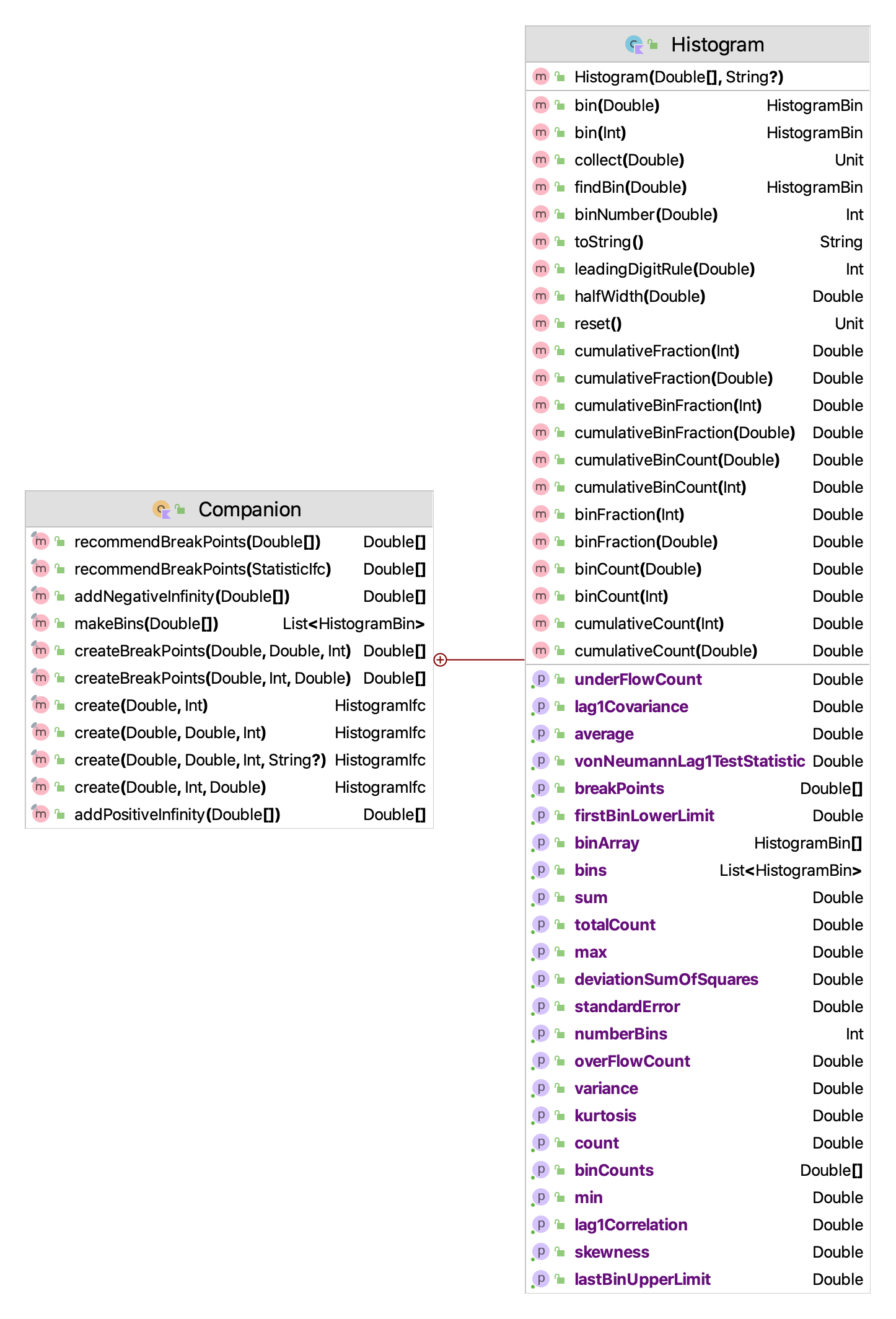
Figure 3.4: Histogram Class
Figure 3.4 presents the methods of the Histogram class. The Histogram class is utilized in a very similar manner as the Statistic class by collecting observations. The observations are then tabulated into the bins. The Histogram class allows the user to tabulate the bin contents via the collect() methods inherited from the AbstractStatistic base class. Since data may fall below the first bin and after the last bin, the implementation also provides counts for those occurrences. Since a Histogram is a sub-class of AbstractStatistic, it also implements the StatisticIfc to provide summary statistics on the data tabulated within the bins.
In some cases, the client may not know in advance the appropriate settings for the number of bins or the width of the bins. In this situation, one can use the recommendBreakPoints function, which uses an array of data or statistics computed on the data. The function recommendBreakPoints computes a reasonable lower limit, number of bins, and bin width based on the statistics.
Example 3.2 (Histograms and Breakpoints) This example illustrates how to configure the breakpoints for a histogram and to use the histogram to observe observations from a random sample.
fun main() {
    val d = ExponentialRV(2.0, streamNum = 1)
    val data = d.sample(1000)
    var bp = Histogram.recommendBreakPoints(data)
    bp = Histogram.addPositiveInfinity(bp)
    val h = Histogram(breakPoints = bp)
    for (x in data) {
        h.collect(x)
    }
    println(h)
    val plot = h.histogramPlot()
    plot.showInBrowser("Exponentially Distributed Data")
}
Histogram: ID_4
-------------------------------------
Number of bins = 25
First bin starts at = 0.0
Last bin ends at = Infinity
Under flow count = 0.0
Over flow count = 0.0
Total bin count = 1000.0
Total count = 1000.0
-------------------------------------
Bin Range Count CumTot Frac CumFrac
1 [ 0.00, 0.75) = 333 333.0 0.333000 0.333000
2 [ 0.75, 1.50) = 198 531.0 0.198000 0.531000
3 [ 1.50, 2.25) = 150 681.0 0.150000 0.681000
4 [ 2.25, 3.00) = 112 793.0 0.112000 0.793000
5 [ 3.00, 3.75) = 75 868.0 0.075000 0.868000
6 [ 3.75, 4.50) = 48 916.0 0.048000 0.916000
7 [ 4.50, 5.25) = 28 944.0 0.028000 0.944000
8 [ 5.25, 6.00) = 19 963.0 0.019000 0.963000
9 [ 6.00, 6.75) = 16 979.0 0.016000 0.979000
10 [ 6.75, 7.50) = 1 980.0 0.001000 0.980000
11 [ 7.50, 8.25) = 5 985.0 0.005000 0.985000
12 [ 8.25, 9.00) = 2 987.0 0.002000 0.987000
13 [ 9.00, 9.75) = 4 991.0 0.004000 0.991000
14 [ 9.75,10.50) = 1 992.0 0.001000 0.992000
15 [10.50,11.25) = 2 994.0 0.002000 0.994000
16 [11.25,12.00) = 1 995.0 0.001000 0.995000
17 [12.00,12.75) = 3 998.0 0.003000 0.998000
18 [12.75,13.50) = 0 998.0 0.000000 0.998000
19 [13.50,14.25) = 0 998.0 0.000000 0.998000
20 [14.25,15.00) = 0 998.0 0.000000 0.998000
21 [15.00,15.75) = 0 998.0 0.000000 0.998000
22 [15.75,16.50) = 1 999.0 0.001000 0.999000
23 [16.50,17.25) = 0 999.0 0.000000 0.999000
24 [17.25,18.00) = 1 1000.0 0.001000 1.000000
25 [18.00,Infinity) = 0 1000.0 0.000000 1.000000
-------------------------------------
Statistics on data collected within bins:
-------------------------------------
ID 5
Name ID_4_Statistics
Number 1000.0
Average 1.9216605939547684
Standard Deviation 1.968265908806584
Standard Error 0.06224203312690073
Half-width 0.12214010773960152
Confidence Level 0.95
Confidence Interval [1.7995204862151668, 2.04380070169437]
Minimum 9.561427092951219E-4
Maximum 17.40419059595123
Sum 1921.6605939547685
Variance 3.8740706877702076
Deviation Sum of Squares 3870.1966170824376
Last value collected 8.548639846481285
Kurtosis 10.67406304701379
Skewness 2.5031667132444806
Lag 1 Covariance -0.12649071302321163
Lag 1 Correlation -0.032683278277103954
Von Neumann Lag 1 Test Statistic -0.8438384394483673
Number of missing observations 0.0
Lead-Digit Rule(1) -2
-------------------------------------Because it may be challenging to specify the breakpoints for a histogram, the KSL also provides the CachedHistogram class, which stores the observed data within a data cache (array) until sufficient data has been observed to provide reasonable breakpoints. The default size of the cache is 512 observations. If less than the cache size is observed, the KSL attempts to find the best breakpoints based on the recommendations found here. The following code illustrates the used of the CachedHistogram class.
fun main() {
    val d = ExponentialRV(2.0, streamNum = 1)
    val data = d.sample(1000)
    val ch = CachedHistogram()
    for (x in data) {
        ch.collect(x)
    }
    println(ch)
    val plot = ch.histogramPlot()
    plot.showInBrowser("Exponentially Distributed Data")
}
The KSL will also tabulate count frequencies when the values are only integers. This is accomplished with the IntegerFrequency class. Figure 3.5 indicates the methods of the IntegerFrequency class. The object can return information on the counts and proportions. It can even create a DEmpiricalCDF distribution based on the observed data.
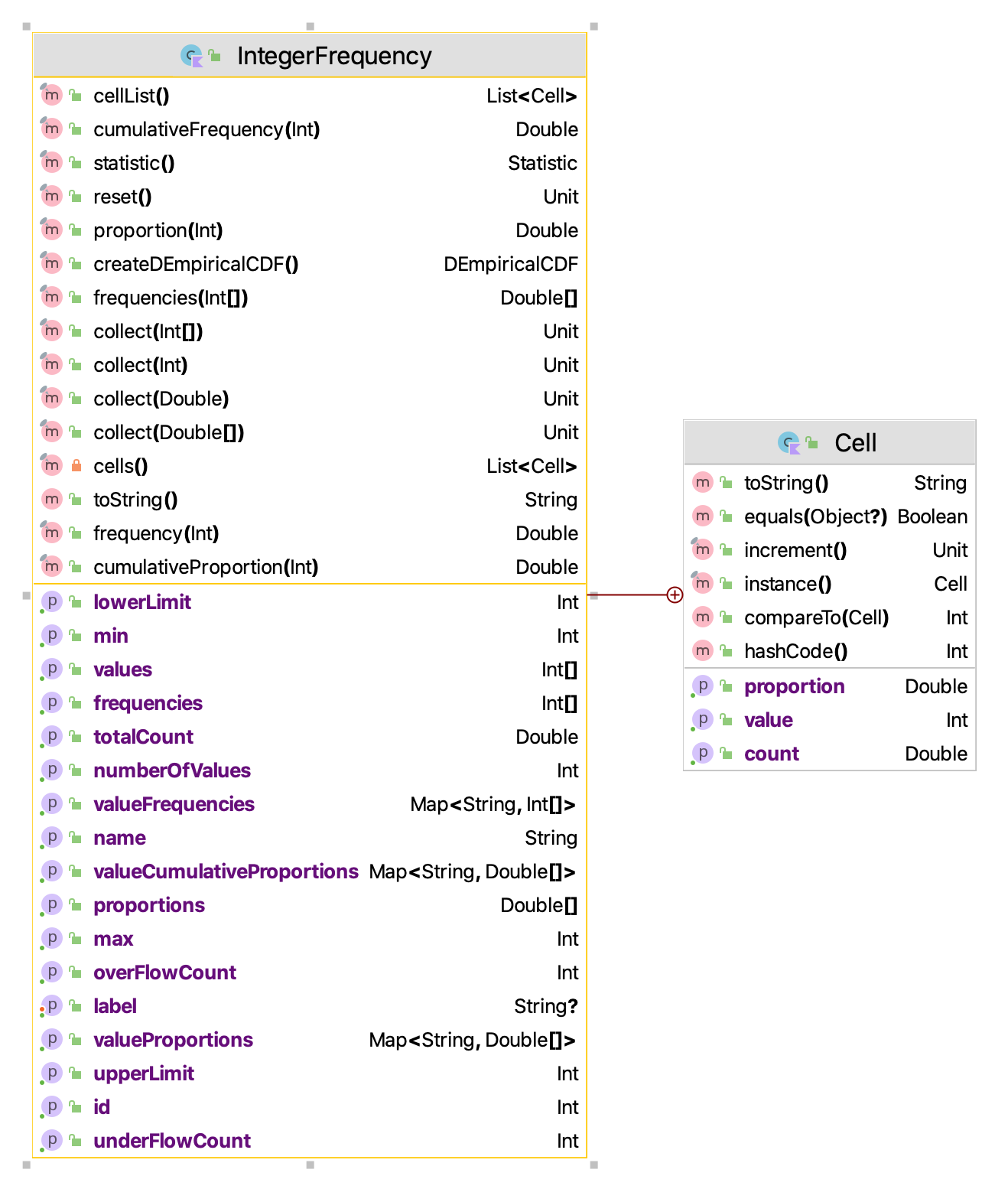
Figure 3.5: IntegerFrequency Class
In the following code example, an instance of the IntegerFrequency class is created. Then, an instance of a binomial random variable is used to generate a sample of 10,000 observations. The sample is then collected by the IntegerFrequency class’s collect() function. Notice the the collect() function can collect observations contained within an array.
Example 3.3 (Integer Frequency Tabulation) In this example, an instance of the IntegerFrequency class is used to tabulate observations from a binomial random variable. A bar chart representation of the frequency is also shown within a browser window.
As can be noted in the output, only those integers that are actually observed are tabulated in terms of the count of the number of times the integer is observed and its proportion. The user does not have to specify the range of possible integers; however, instances of IntegerFrequency can be created that specify a lower and upper limit on the tabulated values. The overflow and underflow counts then tabulate when observations fall outside of the specified range.
Frequency Tabulation Frequency Demo
----------------------------------------
Number of cells = 37
Lower limit = -2147483648
Upper limit = 2147483647
Under flow count = 0
Over flow count = 0
Total count = 10000.0
Minimum value observed = 30
Maximum value observed = 69
----------------------------------------
Value    Count   Proportion
30   1.0     1.0E-4
33   3.0     3.0E-4
34   7.0     7.0E-4
35   10.0    0.001
36   17.0    0.0017
37   23.0    0.0023
38   48.0    0.0048
39   86.0    0.0086
40   101.0       0.0101
41   146.0       0.0146
42   221.0       0.0221
43   319.0       0.0319
44   371.0       0.0371
45   470.0       0.047
46   568.0       0.0568
47   684.0       0.0684
48   742.0       0.0742
49   768.0       0.0768
50   769.0       0.0769
51   813.0       0.0813
52   696.0       0.0696
53   680.0       0.068
54   599.0       0.0599
55   505.0       0.0505
56   386.0       0.0386
57   318.0       0.0318
58   237.0       0.0237
59   142.0       0.0142
60   107.0       0.0107
61   68.0    0.0068
62   38.0    0.0038
63   23.0    0.0023
64   13.0    0.0013
65   14.0    0.0014
66   4.0     4.0E-4
67   2.0     2.0E-4
69   1.0     1.0E-4
----------------------------------------
Finally, the KSL provides the ability to define labeled states and to tabulate frequencies and proportions related to the visitation and transition between the states. This functionality is available in the StateFrequency class. The following code example creates an instance of StateFrequency by providing the number of states. The states are returned in a List and then 10,000 states are randomly selected from the list with equal probability using the KSLRandom functionality to randomly select from lists. The randomly selected state is then observed via the collect() method. State frequency tabulation can be useful within the context of a Markov Chain analysis.
Example 3.4 (State Frequency Tabulation) This example creates six states via the constructor parameter to the StateFrequency class. Then, the KSLRandom functionality to randomly select from a list is used to generate 10000 observations of the next state. Finally, a bar chart representation of the state frequency is also shown within a browser window.
The output is what you would expect based on selecting the states with equal probability. Notice that the StateFrequency class not only tabulates the visits to the states, similar to IntegerFrequency, it also counts and tabulates the transitions between states. These detailed tabulations are available via the various methods of the class. See the documentation for further details.
State Frequency Tabulation for: Identity#1
State Labels
State{id=1, number=0, name='State:0'}
State{id=2, number=1, name='State:1'}
State{id=3, number=2, name='State:2'}
State{id=4, number=3, name='State:3'}
State{id=5, number=4, name='State:4'}
State{id=6, number=5, name='State:5'}
State transition counts
[288, 272, 264, 282, 265, 286]
[283, 278, 283, 286, 296, 266]
[286, 298, 263, 264, 247, 282]
[271, 263, 275, 279, 280, 294]
[274, 305, 273, 281, 296, 268]
[254, 277, 282, 270, 313, 255]
State transition proportions
[0.17380808690404345, 0.16415208207604104, 0.15932407966203982, 0.17018708509354255, 0.15992757996378998, 0.17260108630054316]
[0.16725768321513002, 0.16430260047281323, 0.16725768321513002, 0.1690307328605201, 0.17494089834515367, 0.15721040189125296]
[0.174390243902439, 0.18170731707317073, 0.1603658536585366, 0.16097560975609757, 0.15060975609756097, 0.1719512195121951]
[0.16305655836341756, 0.1582430806257521, 0.1654632972322503, 0.16787003610108303, 0.1684717208182912, 0.17689530685920576]
[0.1614614024749558, 0.17972893341190335, 0.16087212728344136, 0.16558632881555688, 0.17442545668827342, 0.15792575132586917]
[0.15384615384615385, 0.16777710478497881, 0.17080557238037553, 0.16353725015142337, 0.18958207147183526, 0.15445184736523318]

Frequency Tabulation Identity#1
----------------------------------------
Number of cells = 6
Lower limit = 0
Upper limit = 5
Under flow count = 0
Over flow count = 0
Total count = 10000
----------------------------------------
Value    Count   Proportion
0    1657    0.1657
1    1693    0.1693
2    1640    0.164
3    1662    0.1662
4    1697    0.1697
5    1651    0.1651
----------------------------------------
3.1.3 Batch Statistics
In simulation, we often collect data that is correlated. That is, the data have a dependence structure. This causes difficulty in developing valid confidence intervals for the estimators as well as invalidated a number of other statistical procedures that require independent observations. Grouping the data into batches and computing the average of each batch is one methodology for mitigating the effect of dependence within the data on statistical inference procedures. The idea is that the average associated with each batch will tend to be less dependent, especially the larger the batch size. The method of batch means provides a mechanism for developing an estimator for \(Var\lbrack \bar{X} \rbrack\).
The method of batch means is based on observations \((X_{1}, X_{2}, X_{3}, \dots, X_{n})\). The idea is to group the output into batches of size, \(b\), such that the averages of the data within a batch are more nearly independent and possibly normally distributed.
\[\begin{multline*} \underbrace{X_1, X_2, \ldots, X_b}_{batch 1} \cdots \underbrace{X_{b+1}, X_{b+2}, \ldots, X_{2b}}_{batch 2} \cdots \\ \underbrace{X_{(j-1)b+1}, X_{(j-1)b+2}, \ldots, X_{jb}}_{batch j} \cdots \underbrace{X_{(k-1)b+1}, X_{(k-1)b+2}, \ldots, X_{kb}}_{batch k} \end{multline*}\]
Let \(k\) be the number of batches each of size \(b\), where, \(b = \lfloor \frac{n}{k}\rfloor\). Define the \(j^{th}\) batch mean (average) as:
\[ \bar{X}_j(b) = \dfrac{1}{b} \sum_{i=1}^b X_{(j-1)b+i} \] Each of the batch means are treated like observations in the batch means series. For example, if the batch means are re-labeled as \(Y_j = \bar{X}_j(b)\), the batching process simply produces another series of data, (\(Y_1, Y_2, Y_3, \ldots, Y_k\)) which may be more like a random sample. Why should they be more independent? Typically, in auto-correlated processes the lag-k auto-correlations decay rapidly as \(k\) increases. Since, the batch means are formed from batches of size \(b\), provided that \(b\) is large enough the data within a batch is conceptually far from the data in other batches. Thus, larger batch sizes are good for ensuring independence; however, as the batch size increases the number of batches decreases and thus variance of the estimator will increase.
To form a \((1 - \alpha)\)% confidence interval, we simply treat this new series like a random sample and compute approximate confidence intervals using the sample average and sample variance of the batch means series:
\[
\bar{Y}(k) = \dfrac{1}{k} \sum_{j=1}^k Y_j
\]
The sample variance of the batch process is based on the \(k\) batches:
\[
S_b^2 (k) = \dfrac{1}{k - 1} \sum_{j=1}^k (Y_j - \bar{Y}^2)
\]
Finally, if the batch process can be considered independent and identically distributed the \(1-\alpha\) level confidence interval can be written as follows:
\[
\bar{Y}(k) \pm t_{\alpha/2, k-1} \dfrac{S_b (k)}{\sqrt{k}}
\]
The BatchStatistic class within the statistic package implements a basic batching process. The BatchStatistic class works with data as it is presented to its collect method. Since we do not know in advance how much data we have, the BatchStatistic class has rules about the minimum number of batches and the size of batches that can be formed. Theory indicates that we do not need to have a large number of batches and that it is better to have a relatively small number of batches that are large in size.
Three properties of the BatchStatistic class that are important are:
minNumBatches– This represents the minimum number of batches required. The default value for this attribute is determined byBatchStatistic.MIN_NUM_BATCHES, which is set to 20.minBatchSize– This represents the minimum size for forming initial batches. The default value for this attribute is determined byBatchStatistic.MIN_NUM_OBS_PER_BATCH, which is set to 16.maxNumBatchesMultiple– This represents a multiple of minimum number of batches which is used to determine the upper limit (maximum) number of batches. For example, ifmaxNumBatchesMultiple = 2and theminNumBatches = 20, then the maximum number of batches we can have is 40 (2*20). The default value for this property is determined byBatchStatistic.MAX_BATCH_MULTIPLE, which is set to 2.
The BatchStatistic class uses instances of the Statistic class to do its calculations. The bulk of the processing is done in two methods, collect() and collectBatch(). The collect() method simply uses an instance of the Statistic class (myStatistic) to collect statistics. When the amount of data collected (myStatistic.count) equals the current batch size (currentBatchSize) then the collectBatch() method is called to form a batch.
    override fun collect(obs: Double) {
        super.collect(obs)
        myTotNumObs = myTotNumObs + 1.0
        myValue = obs
        myStatistic.collect(myValue)
        if (myStatistic.count == currentBatchSize.toDouble()) {
            collectBatch()
        }
    }
Referring to the collectBatch() method in the following code, the batches that are formed are recorded in an array called bm. After recording the batch average, the statistic is reset for collecting the next batch of data. The number of batches is recorded and if this has reached the maximum number of batches (as determined by the batch multiple calculation), we rebatch the batches back down to the minimum number of batches by combining adjacent batches according to the batch multiple.
    private fun collectBatch() {
        // increment the current number of batches
        numBatches = numBatches + 1
        // record the average of the batch
        bm[numBatches] = myStatistic.average
        // collect running statistics on the batches
        myBMStatistic.collect(bm[numBatches])
        // reset the within batch statistic for next batch
        myStatistic.reset()
        // if the number of batches has reached the maximum then rebatch down to
        // min number of batches
        if (numBatches == maxNumBatches) {
            numRebatches++
            currentBatchSize = currentBatchSize * minNumBatchesMultiple
            var j = 0 // within batch counter
            var k = 0 // batch counter
            myBMStatistic.reset() // clear for collection across new batches
            // loop through all the batches
            for (i in 1..numBatches) {
                myStatistic.collect(bm[i]) // collect across batches old batches
                j++
                if (j == minNumBatchesMultiple) { // have enough for a batch
                    //collect new batch average
                    myBMStatistic.collect(myStatistic.average)
                    k++ //count the batches
                    bm[k] = myStatistic.average // save the new batch average
                    myStatistic.reset() // reset for next batch
                    j = 0
                }
            }
            numBatches = k // k should be minNumBatches
            myStatistic.reset() //reset for use with new data
        }
    }
There are a variety of procedures that have been developed that will automatically batch the data as it is collected. The KSL has a batching algorithm based on the procedure implemented within the Arena simulation language. When a sufficient amount of data has been collected batches are formed. As more data is collected, additional batches are formed until \(k=40\) batches are collected. When 40 batches are formed, the algorithm collapses the number of batches back to 20, by averaging each pair of batches. This has the net effect of doubling the batch size. This process is repeated as more data is collected, thereby ensuring that the number of batches is between 20 and 39. In addition, the procedure also computes the lag-1 correlation so that independence of the batches can be tested.
The BatchStatistic class also provides a public reformBatches() method to allow the user to rebatch the batches to a user supplied number of batches. Since the BatchStatistic class implements the StatisticalAccessorIfc interface, it can return the sample average, sample variance, minimum, maximum, etc. of the batches. Within the discrete-event modeling constructs of the KSL, batching can be turned on to collect batch statistics during a replication. The use of these constructs will be discussed when the discrete-event modeling elements of the KSL are presented.
The following code illustrates how to create and use a BatchStatistic.
Example 3.5 (Batch Statistic Collection) This example code illustrates how to configure an instance of the BatchStatistic class to collect and report statistics associated with the batching process.
fun main() {
    val d = ExponentialRV(2.0)

    // number of observations
    val n = 1000

    // minimum number of batches permitted
    // there will not be less than this number of batches
    val minNumBatches = 40

    // minimum batch size permitted
    // the batch size can be no smaller than this amount
    val minBatchSize = 25

    // maximum number of batch multiple
    //  The multiple of the minimum number of batches
    //  that determines the maximum number of batches
    //  e.g. if the min. number of batches is 20
    //  and the max number batches multiple is 2,
    //  then we can have at most 40 batches
    val maxNBMultiple = 2

    // In this example, since 40*25 = 1000, the batch multiple does not matter
    val bm = BatchStatistic(minNumBatches, minBatchSize, maxNBMultiple)
    for (i in 1..n) {
        bm.collect(d.value)
    }
    println(bm)
    val bma = bm.batchMeans
    var i = 0
    for (x in bma) {
        println("bm($i) = $x")
        i++
    }

    // this re-batches the 40 down to 10
    val reformed = bm.reformBatches(10)
    println(Statistic(reformed))
}
3.1.4 Statistics Summary
The ksl.utilities.statistic package defines a lot of functionality. Here is a summary of some of the useful classes and interfaces.
CollectorIfcdefines a set of collect() methods for collecting data. The method is overridden to permit the collection of a wide variety of data types. The collect() method is designed to collect values and a weight associated with the value. This allows the collection of weighted statistics.Collectoris an abstract base class for building concrete sub-classes.DoubleArraySaverdefines methods for saving observed data to arrays.WeightedStatisticIfcdefines statistics that are computed on weighted data values.WeightedStatisticis a concrete implementation of the interface.AbstractStatisticis an abstract base class for defining statistics. Sub-classes ofAbstractStatisticcompute summary statistics of some kind.Histogramdefines a class to collect statistics and tabulate data into bins.Statisticis a concrete implementation ofAbstractStatisticallowing for a multitude of summary statistics.BatchStatisticis also a concrete implementation ofAbstractStatisticthat provides for summarizing data via a batching process.IntegerFrequencytabulates integer values into a frequencies by observed values, similar to a histogram.StateFrequencyfacilitates defining labeled states and tabulating visitation and transition statistics.StatisticXYcollects statistics on \((x,y)\) pairs computing statistics on the \(x\) and \(y\) values separately, as well as the covariance and correlation between the observations within a pair.BoxPlotSummaryproduces the summary statistics necessary for the construction of a box plot.OLSRegression,RegressionResultsIfc,andRegressionDatafacilitate performing multiple variable regression. The basic use of these classes is illustrated in Section 10.1.4 of Chapter 10.BootstrapSamplerfacilitates the bootstrap statistical analysis technique. Its use is describe in Section 9.1 of Chapter 9.
The most important class within the statistics package is probably the
Statistic class. This class summarizes the observed data into summary
statistics such as: minimum, maximum, average, variance, standard
deviation, lag-1 correlation, and count. In addition, confidence
intervals can be formed on the observations based on the student-t
distribution. Finally, there are useful companion object methods for computing
statistics on arrays and for estimating sample sizes. The reader is
encourage to review the KSL documentation for all of the functionality,
including the ability to write nicely printed statistical results.
In the remaining sections of this chapter, we will illustrate the collection of statistics on simple Monte Carlo models. This begins in the next section by estimating the area of a simple one-dimensional function.