8.2 Constrained Transfer with Movable Resources
A movable resource refers to one or more identical resources that can be allocated to an entity for the purpose of moving entities between locations. The travel time between locations depends on distance and speed.
The standard delay() function assumes no resource constrained transfer. As indicated in the last section, the situation of a general resource being used for the transfer can be easily modeled. In that situation, the time of the transfer was specified. In the case of movable resources, resource constrained transfer is still being modeled, but in addition, the physical distance of the transfer is explicitly modeled. In essence, rather than specifying a time to transfer, you specify a velocity and a distance for the transfer. From the velocity and distance associated with the transfer, the time of the transfer can be computed. In these situations, the physical device and its movement (with or without the entity) through the system is of key interest within the modeling.
The modeling of a resource that moves needs to include the following aspects:
- movement of the resource (empty) to the origin location for pick up
- movement of the resource (not empty) to the destination location for drop off
Besides these two aspects, there are natural modeling enhancements that might be considered:
- time to load the entity for the pick up
- time to unload the entity for the drop off
- possible movement of the resource to a home location after drop off
The KSL models this situation using movable resources with a spatial model.
8.2.1 Spatial Models
A spatial model represents the physical space associated with the environment. For the purposes of
movable resources, a spatial model provides the distance between locations. The KSL supports
a variety of spatial models. The simplest spatial model is probably the DistancesModel class.
Figure 8.3 illustrates the main classes for spatial models. A spatial model
holds spatial elements. Spatial elements are objects that implement the SpatialElementIfc interface.
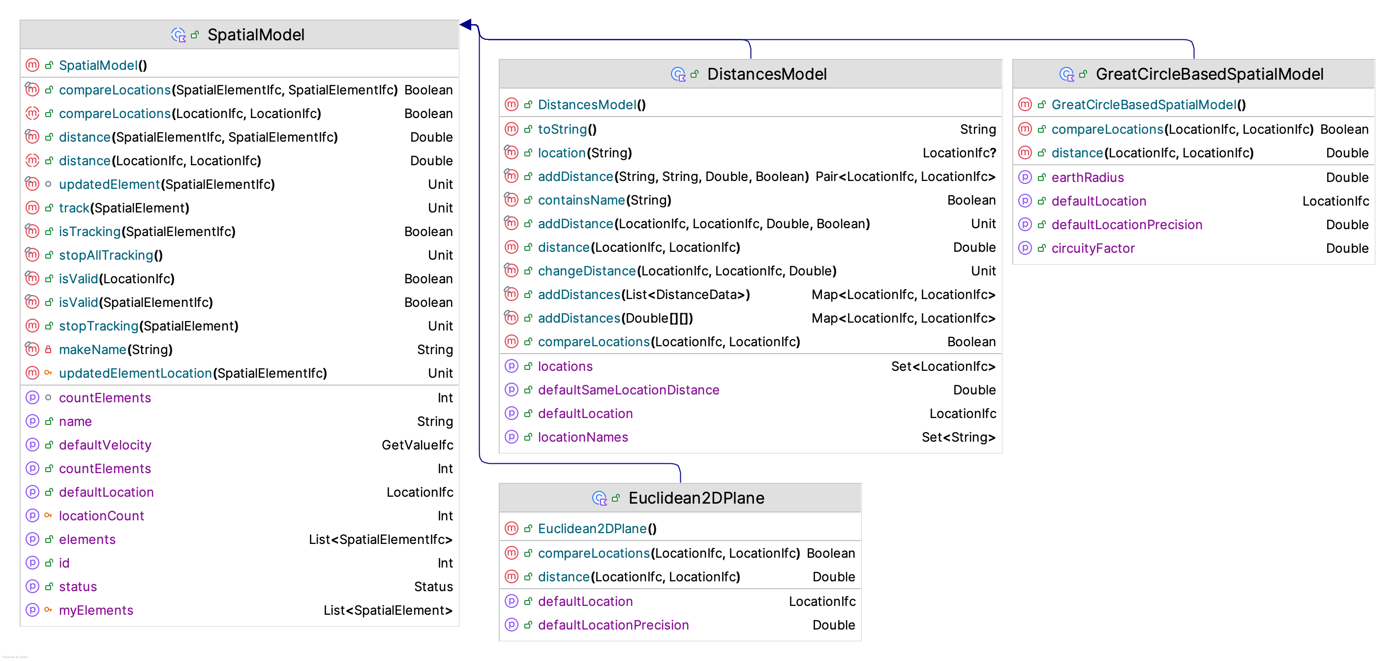
Figure 8.3: Spatial Models
The SpatialModel class is an abstract base class. The key abstract concepts that need to be
implemented by sub-classes are:
    /**
     *  The default initial location.
     */
    abstract var defaultLocation: LocationIfc

    /**
     * Computes the distance between [fromLocation] and [toLocation] based on
     * the spatial model's distance metric
     * @return the distance between the two locations
     */
    abstract fun distance(fromLocation: LocationIfc, toLocation: LocationIfc): Double

    /**
     * Returns true if [firstLocation] is the same as [secondLocation]
     * within the underlying spatial model. This is not object reference
     * equality, but rather whether the locations within the underlying
     * spatial model can be considered spatially (equivalent) according to the model.
     * This may or may not imply that the distance between the locations is zero.
     * No assumptions about distance are implied by true.
     *
     * Requirement: The locations must be valid within the spatial model.
     */
    abstract fun compareLocations(firstLocation: LocationIfc, secondLocation: LocationIfc): Boolean
The KSL provides basic spatial model implementations for the following situations.
- Distances - The distance between locations is provided based on an origin-destination matrix.
- Great Circle - A great circle spatial model represents the distance between two coordinates on the earth based on latitude and longitude. It provides an approximate distance of travelling along the great circle between the coordinates. The model implemented within the KSL allows for the adjustment of the distance based on circuity factor. The circuity factor will adjust the distance based on the mode of transport road or rail.
- Euclidean 2D Plane - The distance is based on computing the distance between two points in the Euclidean 2D plane.
- Rectangular Grid - The 2D plane is divided into a grid with the upper left most corner point representing (0,0). The grid is specified based on the width and height divided into a number of rows and columns. This facilitates the moving between the cells of the grid.
The main abstraction for a spatial model is computing the distance between two locations.
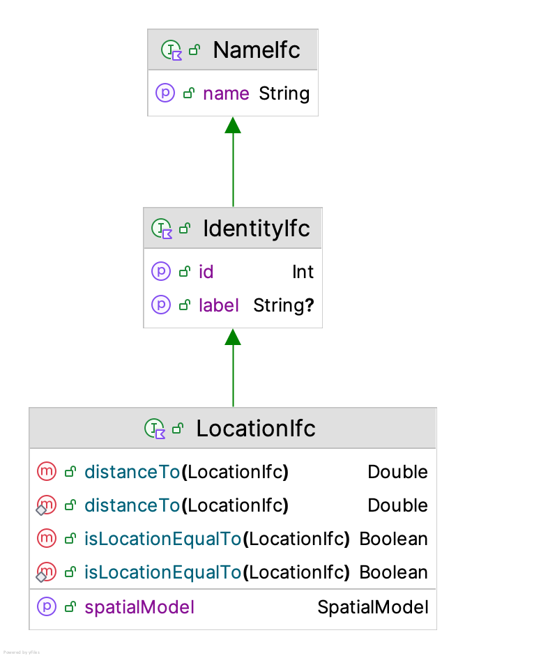
Figure 8.4: Location Interface
A location has a name and an identity. In addition, a location is associated with a spatial model. From the spatial model, a location can compute the distance to other locations within the spatial model. Spatial models are responsible for creating locations and for computing the distance between locations. A spatial model is responsible for defining what constitutes a location. For example, a great circle spatial model uses GPS coordinates to define locations.
As previously mentioned, a basic spatial model is a distances model, which is implemented via the DistancesModel class.
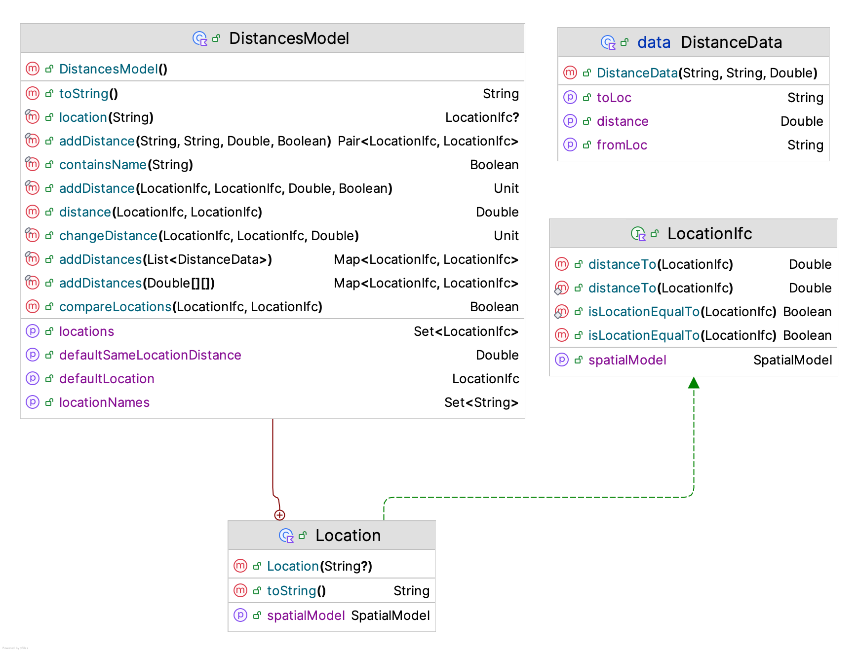
Figure 8.5: Distances Model
In essence, a distance model is a matrix that holds the distances between origins and destinations. Notice from Figure 8.5 that the inner class Location implements the LocationIfc interface for the distance model. The user is responsible for providing the data associated with the locations. The specification can be in the form of matrix or via the data class DistanceData or individually specified via the addDistance() function. The following code illustrates the concepts.
    private val dm = DistancesModel()
    private val enter = dm.Location("Enter")
    private val station1 = dm.Location("Station1")
    private val station2 = dm.Location("Station2")
    private val exit = dm.Location("Exit")

    init {
        // distance is in feet
        dm.addDistance(enter, station1, 60.0, symmetric = true)
        dm.addDistance(station1, station2, 30.0, symmetric = true)
        dm.addDistance(station2, exit, 60.0, symmetric = true)
        dm.addDistance(station2, enter, 90.0, symmetric = true)
        dm.addDistance(exit, station1, 90.0, symmetric = true)
        dm.addDistance(exit, enter, 150.0, symmetric = true)
        dm.defaultVelocity = myWalkingSpeedRV
        spatialModel = dm
    }
In the code, a distances model is created, used to define locations, and then used to specify the distance between locations. As shown in Figure 8.3, a distances model also includes a default velocity because it is a sub-class of the SpatialModel class. Now we are ready to discuss movable resources.
8.2.2 Movable Resources
As mentioned, a movable resource is a resource that moves. The class MovableResource shown in Figure 8.6 is a sub-class of the Resource class, while implementing the SpatialElementIfc and VelocityIfc interfaces. A spatial element is something that can be within a spatial model. Notice that the SpatialElementIfc interface uses locations to specify the initial, previous, and current location of the spatial element.
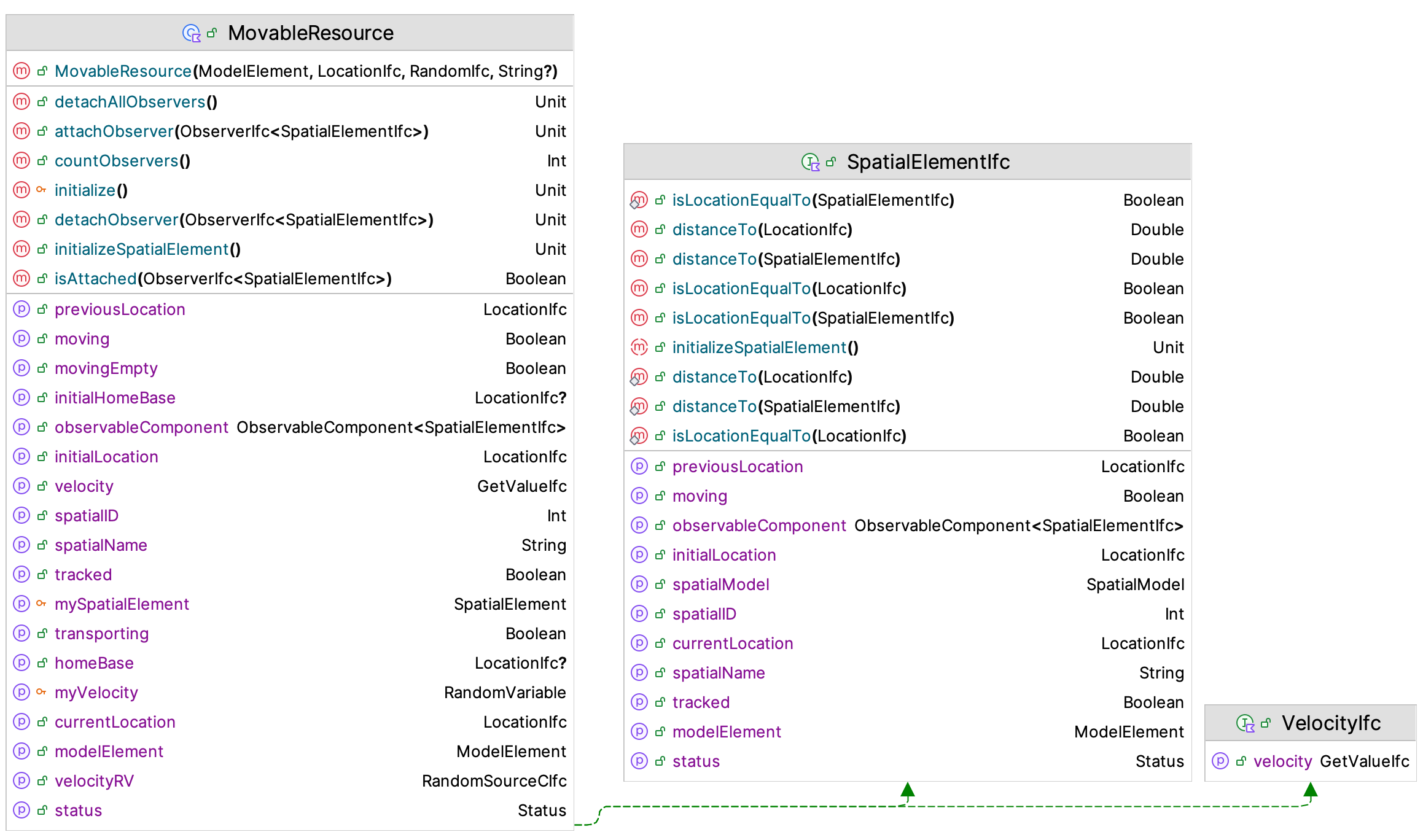
Figure 8.6: Movable Resource
To use movable resources within a process model, we need to define some new suspending functions and discuss how entities keep track of their location. The Entity class implements the SpatialElementIfc interface. Some of the key properties that assist with the use of entities within a spatial model include:
initialLocationThe location of the entity when it is created specified as aLocationIfcinterface instance.previousLocationThe previous location of the entity after it has moved to its current location as specified as aLocationIfcinterface instance.currentLocationThe current location of the entity within the spatial model as specified as aLocationIfcinterface instance.isMovingA boolean property that indicates if the entity is experiencing a movement.velocityA property that implements theGetValueIfcinterface that reports the velocity to use when the entity is moving between locations.
To have entities use movable resources within a process, we need to introduce new suspending functions. To move an entity from one location to another (without a resource), we can use the following variations of the move() function:
move(fromLoc: LocationIfc, toLoc: Location, velocity: Double, movePriority: Int, suspensionName: String?)move(fromLoc: LocationIfc, toLoc: Location, velocity: GetValueIfc, movePriority: Int, suspensionName: String?)
To move something that implements the SpatialElementIfc interface use the following move() function. Note that the entity experiences the delay while the spatial element is moved to the supplied location.
move(spatialElement: SpatialElementIfc, toLoc: Location, velocity: Double, movePriority: Int, suspensionName: String?)
This function uses the spatial element’s current location as the origin. Since movable resources are also spatial elements, we can move them. Again, the entity experiences the time delay associated with the movement of the resource to the supplied location.
move(movableResource: MovableResource, toLoc: Location, velocity: Double, movePriority: Int, suspensionName: String?)move(movableResourceWithQ: MovableResourceWithQ, toLoc: Location, velocity: Double, movePriority: Int, suspensionName: String?)
In addition, we can cause both the entity and a spatial model to move together using variations of the moveWith() function.
moveWith(spatialElement: SpatialElementIfc, toLoc: Location, velocity: Double, movePriority: Int, suspensionName: String?)moveWith(movableResource: MovableResource, toLoc: Location, velocity: Double, movePriority: Int, suspensionName: String?)moveWith(movableResourceWithQ: MovableResourceWithQ, toLoc: Location, velocity: Double, movePriority: Int, suspensionName: String?)
In order to use these functions, the entity and the spatial element must be at the same location. Thus, the standard approach to using a movable resource to move an entity involves first seizing the resource, then moving the resource to the entity’s current location, and finally moving with the resource to the destination. Here is a simple pattern:
val a = seize(movableResource)
move(movableResource, entity.currentLocation, emptyVelocity, emptyMovePriority)
delay(loadingDelay, loadingPriority)
moveWith(movableResource, toLoc, transportVelocity, transportPriority)
delay(unLoadingDelay, unLoadingPriority)
release(a)
In fact, this pattern is so common, there is a suspending function that encapsulates it into one function.
   /**
     *  Causes transport of the entity via the movable resource from the entity's current location to the specified location at
     *  the supplied velocities.
     *  If not specified, the default velocity of the movable resource is used for the movement.
     *  @param movableResource, the spatial element that will be moved
     *  @param toLoc the location to which the entity is supposed to move
     *  @param emptyVelocity the velocity associated with the movement to the entity's location
     *  @param transportVelocity the velocity associated with the movement to the desired location
     *  @param transportQ the queue that the entity waits in if the resource is busy
     *  @param requestPriority, a priority can be used to determine the order of events for
     *  requests for transport
     *  @param emptyMovePriority, since the move is scheduled, a priority can be used to determine the order of events for
     *  moves that might be scheduled to complete at the same time.
     *  @param transportPriority, since the move is scheduled, a priority can be used to determine the order of events for
     *  moves that might be scheduled to complete at the same time.
     */
    suspend fun transportWith(
        movableResource: MovableResource,
        toLoc: LocationIfc,
        emptyVelocity: Double = movableResource.velocity.value,
        transportVelocity: Double = movableResource.velocity.value,
        transportQ: RequestQ,
        loadingDelay: GetValueIfc = ConstantRV.ZERO,
        unLoadingDelay: GetValueIfc = ConstantRV.ZERO,
        requestPriority: Int = TRANSPORT_REQUEST_PRIORITY,
        emptyMovePriority: Int = MOVE_PRIORITY,
        loadingPriority: Int = DELAY_PRIORITY,
        transportPriority: Int = MOVE_PRIORITY,
        unLoadingPriority: Int = DELAY_PRIORITY
    )
NOTE!
The transportWith() function is meant to be a convenience function to cover a standard pattern of usage; however, if your situation varies from the standard pattern, then you can always use the basic move() and moveWith() functions to model a wide variety of situations.
We are now ready to illustrate entity movement and movement using movable resources.
8.2.3 Tandem Queue Model With Movement
Recall the tandem queue model in Example 7.1. For this section, we are going to enhance the example with movement. In this situation, parts will enter the system at a loading dock that is 60 feet from the station staffed by the first worker. For simplicity, let’s assume that there are always plenty of workers available to move the part from the loading dock to the first station. After the part completes processing at station 1, it is moved to station 2. Again, assume that there are plenty of workers available to move the part from station 1 to station 2. The distance from station 1 to station 2 is 30 feet. After completing processing at station 2, the part is moved to a storage area, where it exits the system. The distance from station 2 to the storage area is 60 feet. We can assume that the walking speed of the workers that move the parts is a triangular distributed random variable with a minimum of 88, a mode of 176, and a maximum of 264, all in feet per minute.
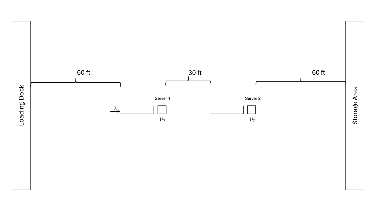
Figure 8.7: Tandem Queue with Distances
To model this situation, we will use the distances spatial model. To implement this situation, we will:
- Use the
Locationclass within theDistancesModelto define locations - Use the
addDistance()function to specify the distance between two locations - Use the
spatialModelproperty to specify the spatial model used by theProcessModel
Let’s start by defining the distances via the DistancesModel class. In the following code, the DistancesModel instance is created
and then used to create the four locations within the spatial model’s context. Then, the init block is used to add the distance
data to the model.
class TandemQueueWithUnConstrainedMovement(
  parent: ModelElement,
  name: String? = null
) : ProcessModel(parent, name) {

    // velocity is in feet/min
    private val myWalkingSpeedRV = TriangularRV(88.0, 176.0, 264.0)
    private val dm = DistancesModel()
    private val enter = dm.Location("Enter")
    private val station1 = dm.Location("Station1")
    private val station2 = dm.Location("Station2")
    private val exit = dm.Location("Exit")

    init {
        // distance is in feet
        dm.addDistance(enter, station1, 60.0, symmetric = true)
        dm.addDistance(station1, station2, 30.0, symmetric = true)
        dm.addDistance(station2, exit, 60.0, symmetric = true)
        dm.defaultVelocity = myWalkingSpeedRV
        spatialModel = dm
    }
Notice that the distances are assumed to be symmetric. That is the distance from the enter location to the station1 location is the same (60 feet) in both directions. The line dm.defaultVelocity = myWalkingSpeedRV indicates that whenever a velocity is needed for a movement, the walking speed distribution is used. Finally, the line spatialModel = dm causes the process model to use the distances model for its spatial model. This ensures that the entities created within the process model will use the distances model as their spatial model context. Once distances have been defined the tandem queue system movement can be easily handled within the process description.
    private inner class Customer : Entity() {
        val tandemQProcess: KSLProcess = process(isDefaultProcess = true) {
            currentLocation = enter
            wip.increment()
            timeStamp = time
            moveTo(station1)
            use(worker1, delayDuration = st1)
            moveTo(station2)
            use(worker2, delayDuration = st2)
            moveTo(exit)
            timeInSystem.value = time - timeStamp
            wip.decrement()
        }
    }
Notice the setting of the entity’s currentLocation in the first line of the process. This line ensures that the entity is located at the enter location when it starts the process. The current location property will be updated by the moveTo() functions so that after the movement, the entity’s location is the destination of the movement. The results of running the model with the additional movement indicate that the movement affects the time spent in the system.
Name                                 Count        Average      Half-Width
--------------------------------------------------------------------------
worker1:InstantaneousUtil             30           0.6982          0.0023
worker1:NumBusyUnits                  30           0.6982          0.0023
worker1:ScheduledUtil                 30           0.6982          0.0023
worker1:WIP                           30           2.2966          0.0388
worker1:Q:NumInQ                      30           1.5983          0.0371
worker1:Q:TimeInQ                     30           1.6001          0.0356
worker2:InstantaneousUtil             30           0.8984          0.0037
worker2:NumBusyUnits                  30           0.8984          0.0037
worker2:ScheduledUtil                 30           0.8984          0.0037
worker2:WIP                           30           8.5321          0.4317
worker2:Q:NumInQ                      30           7.6337          0.4289
worker2:Q:TimeInQ                     30           7.6378          0.4190
TandemQModel:NumInSystem              30          11.7191          0.4414
TandemQModel:TimeInSystem             30          11.7288          0.4250
worker1:SeizeCount                    30       14981.8667         40.6211
worker2:SeizeCount                    30       14979.4667         41.3926
-------------------------------------------------------------------------
In the previous example, we assumed that there was an unlimited number of workers available to move the parts. This results in only a simple delay time to move from one location to another. Now, let’s make the more realistic assumption that in order to move a finite number of workers are available such that when a part needs to move between the stations one of the workers dedicated to the transport task must be available to move the part; otherwise the part must wait until a transport worker is available. For simplicity, we are going to assume that their are 3 transport workers, with one dedicated to moving parts to station 1, another dedicated to moving parts from station 1 to station 2, and the third worker dedicated to moving parts from the third workstation to storage. We are also going to assume that the transport worker stays at the drop off location until requested for its next movement.
Because the transport workers stay at the drop off location, we may need to consider two-way travel. Also, we will need to consider where the transport workers are located at the start of the simulation. We are going to assume that the transport workers all start at the enter location. These assumptions will require an update to the distances. Why? Because we now need to account for the distance to move empty.
    private val myWalkingSpeedRV = TriangularRV(88.0, 176.0, 264.0)
    private val dm = DistancesModel()
    private val enter = dm.Location("Enter")
    private val station1 = dm.Location("Station1")
    private val station2 = dm.Location("Station2")
    private val exit = dm.Location("Exit")

    init {
        // distance is in feet
        dm.addDistance(enter, station1, 60.0, symmetric = true)
        dm.addDistance(station1, station2, 30.0, symmetric = true)
        dm.addDistance(station2, exit, 60.0, symmetric = true)
        dm.addDistance(station2, enter, 90.0, symmetric = true)
        dm.addDistance(exit, station1, 90.0, symmetric = true)
        dm.addDistance(exit, enter, 150.0, symmetric = true)
        dm.defaultVelocity = myWalkingSpeedRV
        spatialModel = dm
    }
Notice that we need to specify the distance from the station2 location to the enter location. This is because the movable resource will be at the enter location at the start of the simulation and will need to move to the station2 location for a pick up. This movement (as well as others) occur because the resource must move to the pick up location (empty) and because the resource stays at the location of the drop off. Now, we can define the movable resources.
   private val mover1: MovableResourceWithQ = MovableResourceWithQ(this, enter, myWalkingSpeedRV, "Mover1")
   private val mover2: MovableResourceWithQ = MovableResourceWithQ(this, enter, myWalkingSpeedRV, "Mover2")
   private val mover3: MovableResourceWithQ = MovableResourceWithQ(this, enter, myWalkingSpeedRV, "Mover3")
Notice that we define the resources to have a queue. This queue will hold requests for the resource when more than one part requires a move. The process description can now be updated to use the movable resources. The following code explicitly seizes the movable resource, moves the resource to the location of the part, and then moves with the resource before then releasing the resource.
    private inner class Customer : Entity() {
        val tandemQProcess: KSLProcess = process(isDefaultProcess = true) {
            currentLocation = enter
            wip.increment()
            timeStamp = time
            val a1 = seize(mover1)
            move(mover1, toLoc = enter)
            moveWith(mover1, toLoc = station1)
            release(a1)
            use(worker1, delayDuration = st1)
            val a2 = seize(mover2)
            move(mover2, toLoc = station1)
            moveWith(mover2, toLoc = station2)
            release(a2)
            use(worker2, delayDuration = st2)
            val a3 = seize(mover3)
            move(mover3, toLoc = station2)
            moveWith(mover3, toLoc = exit)
            release(a3)
            timeInSystem.value = time - timeStamp
            wip.decrement()
        }
    }
The following code shortens the process by using the transportWith() and use() functions.
    private inner class Customer : Entity() {
        val tandemQProcess: KSLProcess = process(isDefaultProcess = true) {
            currentLocation = enter
            wip.increment()
            timeStamp = time
            transportWith(mover1, station1)
            use(worker1, delayDuration = st1)
            transportWith(mover2, station2)
            use(worker2, delayDuration = st2)
            transportWith(mover3, exit)
            timeInSystem.value = time - timeStamp
            wip.decrement()
        }
    }
Suppose that there is a time required to load and unload the part. Let’s assume that the loading time is uniformly distributed between 0.5 and 0.8 minutes and the unloading time is uniformly distributed between 0.25 and 0.5 minutes. In addition, suppose that the workers the perform the movement are not dedicated to a particular station, but instead, they are in a pool of workers that may perform the pick up and delivery of the parts.
For this situation, we can use an instance of the MovableResourcePoolWithQ class. To define the pool
the following code can be used.
    private val mover1 = MovableResource(this, enter, myWalkingSpeedRV, "Mover1")
    private val mover2 = MovableResource(this, enter, myWalkingSpeedRV, "Mover2")
    private val mover3 = MovableResource(this, enter, myWalkingSpeedRV, "Mover3")
    private val moverList = listOf(mover1, mover2, mover3)
    private val movers = MovableResourcePoolWithQ(this, moverList, myWalkingSpeedRV, name = "Movers")
By using the transportWith() function
we can easily add the loading and unloading time delays as follows:
    private val myLoadingTime = RandomVariable(this, UniformRV(0.5, 0.8))
    val loadingTimeRV: RandomSourceCIfc
        get() = myLoadingTime
    private val myUnLoadingTime = RandomVariable(this, UniformRV(0.25, 0.5))
    val unloadingTimeRV: RandomSourceCIfc
        get() = myUnLoadingTime

    private inner class Customer : Entity() {
        val tandemQProcess: KSLProcess = process(isDefaultProcess = true) {
            currentLocation = enter
            wip.increment()
            timeStamp = time
            transportWith(movers, station1, loadingDelay = myLoadingTime, unLoadingDelay = myUnLoadingTime)
            use(worker1, delayDuration = st1)
            transportWith(movers, station2, loadingDelay = myLoadingTime, unLoadingDelay = myUnLoadingTime)
            use(worker2, delayDuration = st2)
            transportWith(movers, exit, loadingDelay = myLoadingTime, unLoadingDelay = myUnLoadingTime)
            timeInSystem.value = time - timeStamp
            wip.decrement()
        }
    }
A pool of movable resources is essentially a “motor pool” or fleet. An importance aspect of modeling a pool of movable resources is how to dispatch the next movable resource. The concept of pooled resources was discussed in Section 7.1.2. In that section, the need for a resource selection rule was briefly mentioned. Within a spatial context, how the next resource is selected to respond to a request may become important. Recall that a resource selection rule determines the list of resources that have enough capacity available to meet the request. In the context of movable resources, the requested capacity is always one unit. Thus, the resource selection rule returns a list of available resources (not seized). Then, from this list a resource must be selected for allocation. The construction of the list of movable resources for possible allocation is governed by the MovableResourceSelectionRuleIfc interface.
/**
 * Provides for a method to select movable resources from a list such that
 * the returned list will contain movable resources that can satisfy the request
 * or the list will be empty.
 */
fun interface MovableResourceSelectionRuleIfc {
    /**
     * @param list of resources to consider selecting from
     * @return the selected list of resources. It may be empty
     */
    fun selectMovableResources(list: List<MovableResource>): MutableList<MovableResource>
}
By default, the movable resource selection rule is provided by the MovableResourceSelectionRule class, which simply returns all available units for possible allocation. Since the allocation rules selects from this list, it is likely that the default selection rule will work for the vast majority of situations.
Within a spatial context, the resource selected for allocation may need additional consideration. For example, it may make sense to allocate the resource that is closest to the requesting entity. The KSL supports a variety of movable resource allocation rules via the MovableResourceAllocationRuleIfc interface.
/**
 *  Function to determine which movable resource should be allocated to
 *  a request. The function provides the location of the request to allow
 *  distance based criteria to be used.
 */
fun interface MovableResourceAllocationRuleIfc {

    /** The method assumes that the provided list of resources has
     *  enough units available to satisfy the needs of the request.
     *
     * @param requestLocation the location associated with the request. This information can be
     * used to determine the allocation based on distances.
     * @param resourceList list of resources to be allocated from
     * @return the amount to allocate from each resource as a map
     */
    fun selectMovableResourceForAllocation(
        requestLocation: LocationIfc,
        resourceList: MutableList<MovableResource>
    ): MovableResource
}
The KSL provides the following movable resource allocation rules.
ClosestMovableResourceAllocationRule- This rule determines which of the available movable resources is closest to the request’s location. This is the default rule.FurthestMovableResourceAllocationRule- This rule determines which of the available movable resources is furthers from the request’s location. This rule may be useful to return movable resources from the outskirts of the spatial model to more central activities.RandomMovableResourceAllocationRule- This rule randomly selects from the available movable resources. This rule may be useful for a fairer distribution of activity across the resources.MovableResourceAllocateInOrderListedRuleThis rule returns the first available resource from the selected resources.MovableResourceAllocationRule- This rule allows a user to determine the order of allocation based on a user defined comparator. The following comparison based rules are based on this approach.LeastUtilizedMovableResourceAllocationRule- Allocates to the movable resource that is currently the least utilized (based on the utilization statistics). This can be useful if fairness is a criteria.LeastSeizedMovableResourceAllocationRule- Allocates to the movable resource that has been seized (allocated) the least. This can be useful if fairness is a criteria.
The reader will be asked to explore the use of these different rules within the exercises.