2.3 Probability Distribution Models
The ksl.utilities.random.rvariable package is the key package for generating random variables; however, it does not facilitate performing calculations involving the underlying probability distributions. To perform calculations involving probability distributions, you should use the ksl.utilities.distributions package. This package has almost all the same distributions represented within the ksl.utilities.random.rvariable package.

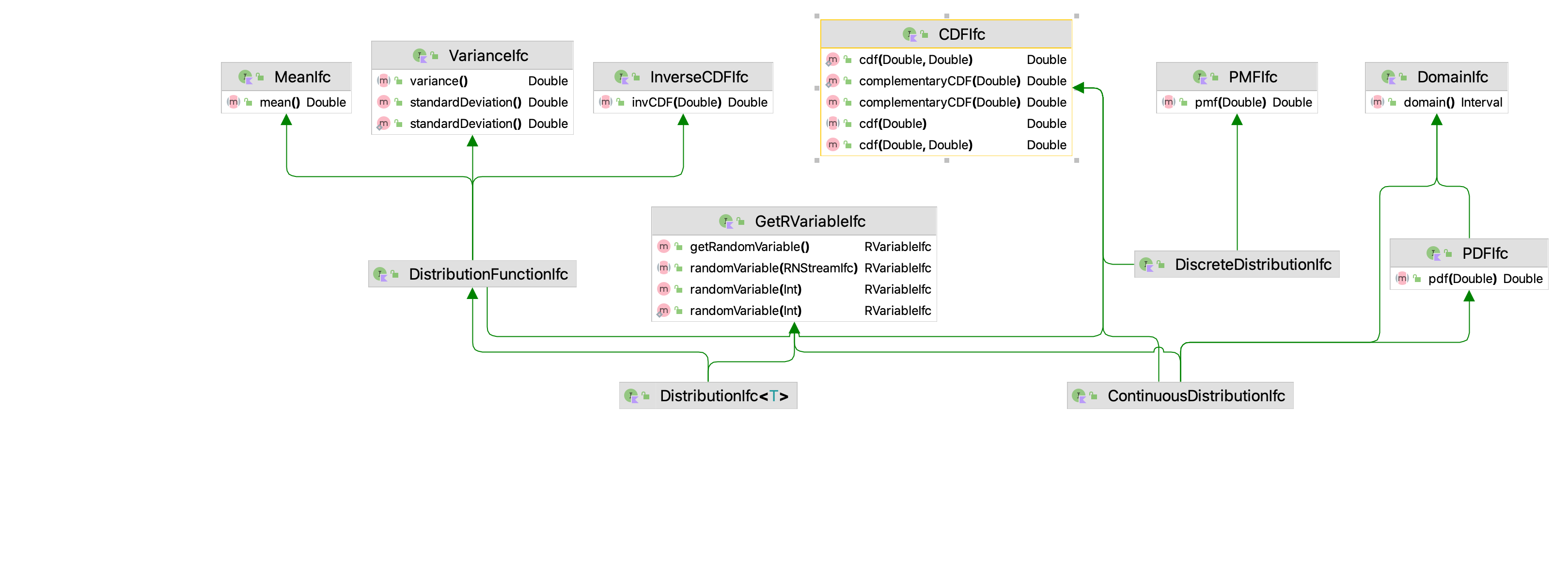
Figure 2.6: Distribution Interfaces
Figure2.6 illustrates the interfaces used to define probability distributions. First, the interface, CDFIfc serves as the basis for discrete distributions via the DiscreteDistributionIfc interface, for continuous distributions via the ContinuousDistributionIfc interface and the general DistributionIfc interface. The discrete distributions such as the geometric, binomial, etc. implement the DiscreteDistributionIfc and PMFIfc interfaces. Similarly, continuous distributions like the normal, uniform, etc. implement the ContinuousDistributionIfc and PDFIfc interfaces. All concrete implementations of distributions extend from the abstract Distribution class, which implements the DistributionIfc interface. Thus, all distributions have the following capabilities:
cdf(b: Double)- computes the cumulative probability, \(F(b) = P(X \leq b)\)cdf(a: Double, b: Double)- computes the cumulative probability, \(P( a \leq X \leq b)\)complementaryCDF(b: Double)- computes the cumulative probability, \(1-F(b) = P(X > b)\)mean()- returns the expected value (mean) of the distributionvariance()- returns the variance of the distributionstandardDeviation()- returns the standard deviation of the distributioninvCDF(p: Double)- returns the inverse of the cumulative distribution function \(F^{-1}(p)\). This is performed by numerical search if necessary
Discrete distributions have a method called pmf(k: Double) that returns the probability associated with the value \(k\). Continuous distributions have a probability density function, \(f(x)\), implemented in the method, pdf(x : Double). Finally, all distributions know how to create random variables through the GetRVariableIfc interface that provides the following methods.
RVariableIfc randomVariable(stream: RNStreamIfc)- returns a new instance of a random variable based on the current values of the distribution’s parameters that uses the supplied streamRVariableIfc randomVariable(streamNum: Int)- returns a new instance of a random variable based on the current values of the distribution’s parameters that uses the supplied stream numberRVariableIfc randomVariable()- returns a new instance of a random variable based on the current values of the distribution’s parameters that uses a newly created stream
As an example, the following code illustrates some calculations for the binomial distribution.
Example 2.22 (Computing with a Binomial Distribution) This example code illustrates how to create a binomial distribution and to use some of its functions to compute the mean, variance, and perform some basic calculations involving probabilities. Notice that the parameters of a distribution can be changes and that distributions can create random variables for generating variates.
fun main() {
    // make and use a Binomial(p, n) distribution
    val n = 10
    val p = 0.8
    println("n = $n")
    println("p = $p")
    val bnDF = Binomial(p, n)
    println("mean = " + bnDF.mean())
    println("variance = " + bnDF.variance())
    // compute some values
    print(String.format("%3s %15s %15s %n", "k", "p(k)", "cdf(k)"))
    for (i in 0..10) {
        print(String.format("%3d %15.10f %15.10f %n", i, bnDF.pmf(i), bnDF.cdf(i)))
    }
    println()
    // change the probability and number of trials
    bnDF.probOfSuccess = 0.5
    bnDF.numTrials = 20
    println("mean = " + bnDF.mean())
    println("variance = " + bnDF.variance())
    // make random variables based on the distributions
    val brv = bnDF.randomVariable(1)
    print(String.format("%3s %15s %n", "n", "Values"))
    // generate some values
    for (i in 1..5) {
        // value property returns generated values
        val x = brv.value.toInt()
        print(String.format("%3d %15d %n", i, x))
    }
}
The output shows the mean, variance, and basic probability calculations.
n = 10
p = 0.8
mean = 8.0
variance = 1.5999999999999996
  k            p(k)          cdf(k)
  0    0.0000001024    0.0000001024
  1    0.0000040960    0.0000041984
  2    0.0000737280    0.0000779264
  3    0.0007864320    0.0008643584
  4    0.0055050240    0.0063693824
  5    0.0264241152    0.0327934976
  6    0.0880803840    0.1208738816
  7    0.2013265920    0.3222004736
  8    0.3019898880    0.6241903616
  9    0.2684354560    0.8926258176
 10    0.1073741824    1.0000000000
The ksl.utilities.random.rvariable package creates instances of random variables that are immutable. That is, once you create a random variable, its parameters cannot be changed. However, distributions permit their parameters to be changed and they also facilitate the creation of random variables. The example code uses the properties probOfSuccess and numTrials to change the parameters of the previously created binomial distribution and then creates a random variable based on the mutated distribution.
mean = 10.0
variance = 5.0
  n          Values
  1               7
  2               9
  3               9
  4              12
  5               8
The results are as we would expect. Similar calculations can be made for continuous distributions. In most cases, the concrete implementations of the various distributions have specialized methods beyond those generic methods described here. Please refer to the documentation for further details.
There are a number of useful companion object methods defined for the binomial, normal, gamma, and Student-T distributions. Specifically, for the binomial distribution, has the following methods
binomialPMF(j: Int, n: Int, p: Double)- directly computes the probability for the value \(j\)binomialCDF(j: Int, n: Int, p: Double)- directly computes the cumulative distribution function for the value \(j\)binomialCCDF(j: Int, n: Int, p: Double)- directly computes the complementary cumulative distribution function for the value of \(j\)binomialInvCDF(x: Double, n: Int, p: Double)- directly computes the inverse cumulative distribution function
These methods are designed to perform their calculations in a numerically stable manner to ensure numerical accuracy. The normal distribution has the following companion object methods for computations involving the standard normal distribution.
stdNormalCDF(z: Double)- the cumulative probability for a \(Z ~ N(0,1)\) random variable, i.e. \(F(z) = P(Z \leq z)\)stdNormalComplementaryCDF(z: Double)- returns \(1-P(Z \leq z)\)stdNormalInvCDF(p: Double)- returns \(z = F^{-1}(p)\) the inverse of the cumulative distribution function
The Student-T distribution also has two convenience methods to facilitate computations.
cdf(dof: Double, x: Double)- computes the cumulative distribution function for \(x\) given the degrees of freedominvCDF(dof: Double, p: Double)- computes the inverse cumulative distribution function or t-value for the supplied probability given the degrees of freedom.
Within the Gamma class’s companion object there are some convenience methods for computing the gamma function, the natural logarithm of the gamma function, the incomplete gamma function, and the digamma function (derivative of the natural logarithm of the gamma function).