8.4 Modeling Systems with Conveyors
A conveyor is a track, belt, or some other device that provides movement over a fixed path. Typically, conveyors are used to transport items that have high volumes over short to medium range distances. The speeds of conveyance typically range from 20-80 feet per minute to as fast as 500 feet per minute. Conveyors can be gravity based or powered. The modeling of conveyors can be roughly classified as follows:
- Accumulating
-
Items on the conveyor continue to move forward when there is a blockage on the conveyor.
- Non-accumulating
-
Items on the conveyor stop when the conveyor stops
- Fixed spacing
-
Items on the conveyor have a fixed space between them or the items ride in a bucket or bin.
- Random spacing
-
Items are placed on the conveyor in no particular position and take up space on the conveyor.
You have experienced conveyors in some form. For example, the belt conveyor at a grocery store is like an accumulating conveyor. An escalator is like a fixed spaced non-accumulating conveyor (the steps are like a bucket for the person to ride in. People movers in airports are like non-accumulating, random spacing conveyors. When designing systems with conveyors there are a number of performance measures to consider:
- Throughput capacity
-
The number of loads processed per time
- Delivery time
-
The time taken to move the item from origin to destination
- Queue lengths
-
The queues to get on the conveyor and for blockages when the conveyor accumulates
- Number of carriers used or the space utilized
-
The number of spaces on the conveyor used
The modeling of conveyors does not necessarily require specialized simulation constructs. For example, gravity based conveyors can be modeled with a deterministic delay. The delay is set to model the time that it takes the entity to fall or slide from one location to another. One simple way to model multiple items moving on a conveyor is to use a resource to model the front of the conveyor with a small delay to load the entity on the conveyor. This allows for spacing between the items on the conveyor. Once on the conveyor the entity releases the front of the conveyor and delays for its move time to the end of the conveyor. At the end of the conveyor, there could be another resource and a delay to unload the conveyor. As long as the delays are deterministic, the entities will not pass each other on the conveyor. If you are not interested in modeling the space taken by the conveyor, then this type of modeling is very reasonable. (Henriksen and Schriber 1986) discuss a number of ways to approach the simulation modeling of conveyors. When space becomes an important element of the modeling, then the simulation language constructs for conveyors become useful. For example, if there actually is a conveyor between two stations and the space allocated for the length of the conveyor is important to the system operation, you might want to use conveyor related constructs.
A conveyor is a material-handling device for transferring or moving entities along a pre-determined path having fixed pre-defined loading and discharge points. Each entity to be conveyed must wait for sufficient space on the conveyor before it can gain entry and begin its transfer. In essence, simulation modeling constructs for conveyors model the travel path via a mapping of space/distance to resources. Space along the path is divided up into units of resources called cells. The conveyor is then essentially a set of moving cells of equal length. Whenever an entity reaches a conveyor entry point it must wait for a predefined amount of unoccupied and available consecutive cells in order to get on the conveyor.
Figure 8.8 illustrates the idea of modeling a conveyor as a set of contiguous cells representing the space on the conveyor. One way to think of this is like an escalator with each cell being a step.
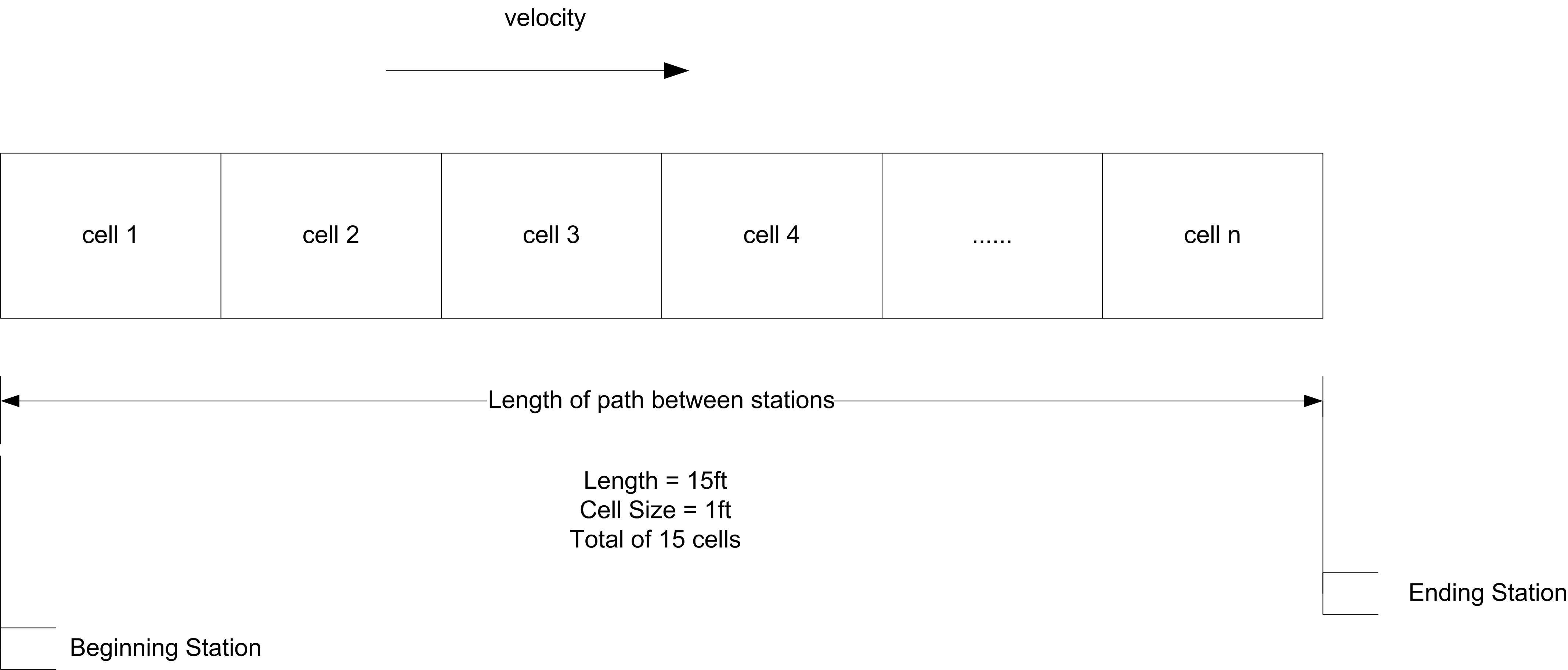
Figure 8.8: A conveyor conceptualized as a set of contiguous cells
In the figure, if each cell represents 1 foot and the total length of the conveyor is 15 feet, then there will be 15 cells. The cell size of the conveyor is the smallest portion of a conveyor that an entity can occupy. In modeling with conveyors, the size of the entity also matters. For example, think of people riding an escalator. Some people have a suitcase and take up two steps and others do not have a suitcase an only take up one step. An entity must acquire enough contiguous cells to hold their physical size in order to be conveyed.
Conveyors travel in a single direction. For non-accumulating conveyors, the spacing remains the same between the entities. When an entity is placed on the conveyor, the entire conveyor is disengaged or stopped until instructions are given to transfer the entity to its destination. When the entity reaches its destination, the entire conveyor is again disengaged until instructions are given to remove the entity from the conveyor, at which time it is engaged or started. Thus, all entities on a non-accumulating conveyor experience the loading and unloading delays of all the other entities.
As previously mentioned, the conveyor is divided into a number of cells. To get on the conveyor and begin moving, the entity must have its required number of contiguous cells. For example, in Figure 8.9, the circle needed 1 cell to get on the conveyor. Suppose the hexagon was trying to get on the conveyor. As cell 2 became available, the hexagon would seize it. Then it would wait for the next cell (cell 1) to become available and seize it. After having both required cells, it is “on” the conveyor. But moving on a conveyor is a bit more continuous than this. Conceptually, you can think of the hexagon, starting to move on the conveyor when it gets cell 2. When one cell moves, all cells must move, in lock step. Since entities are mapped on to the cells by their size, when a cell moves the entity moves. Reversing this analogy becomes useful. Suppose the cells are fixed, but the entities can move. In order for an entity to “take a step” it needs the next cell. As it crosses over to the next cell it releases the previous cell that it occupied. It is as if the entity’s “step size” is 1 cell at a time.

Figure 8.9: Different entity sizes on a conveyor
Figure 8.10 illustrates an approximate
activity flow diagram for an entity using a non-accumulating conveyor.
Suppose the entity size is 2 feet and each cell is 1 foot on the
conveyor. There is a queue for the entities waiting to access the
conveyor. The cells of the conveyor act as resources modeling the space
on the conveyor. The movements of the entity through the space of each
cell are activities. For the 2 foot entity, it first seizes the first
cell and then moves through the distance of the cell. After the movement
it seizes the next cell and moves through its length. Because it is 2
feet (cells) long it seizes the 3rd cell and then releases the first
cell before delaying for the move time for the 3rd cell. As cells become
released other entities can seize them and continue their movement. The
repeated pattern of overlapping seize() and release() function calls that underlie
conveyor modeling clearly depends upon the number of cells and the size
of the entity. Thus, the activity diagram would actually vary by the
size of the entity (number of cells required).
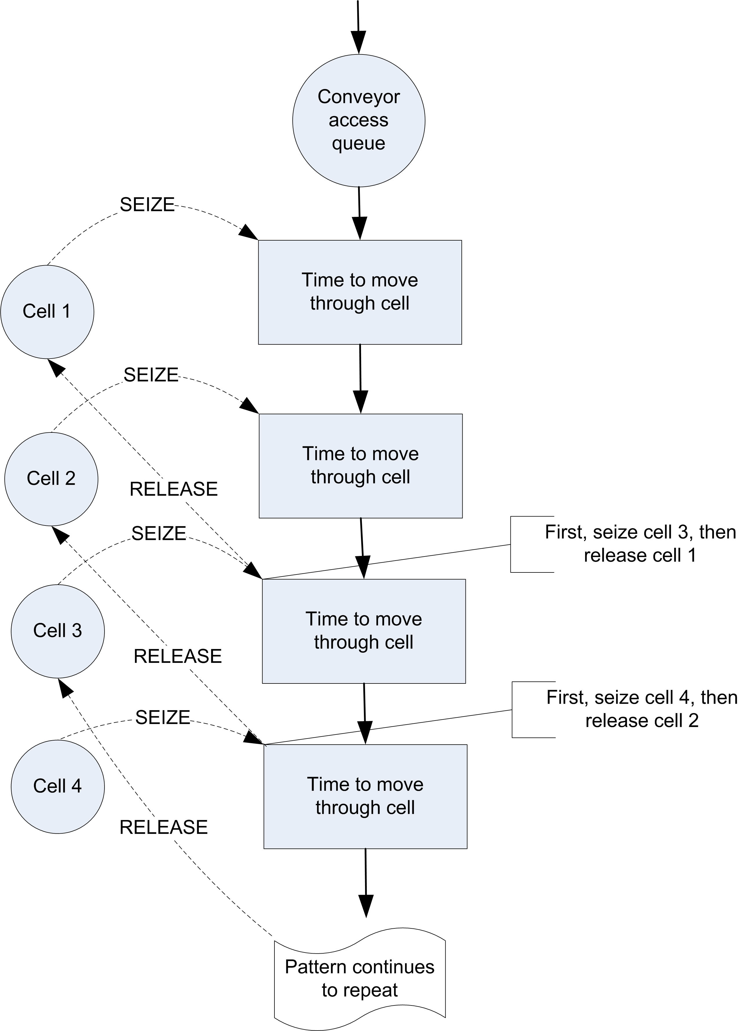
Figure 8.10: Activity diagram for non-accumulating conveyor
The larger the number of cells to model a segment of a conveyor the more slowly the model will execute; however, a larger number of cells allows for a more “continuous" representation of how entities actually exit and leave the conveyor. Larger cell sizes force entities to delay longer to move and thus waiting entities must delay for available space longer. A smaller mapping of cells to distance allows then entity to”creep" onto the conveyor in a more continuous fashion. For example, suppose the conveyor was 6 feet long and space was modeled in inches. That is, the length of the conveyor is 72 inches. Now suppose the entity required 1 foot of space while on the conveyor. If the conveyor is modeled with 72 cells, the entity starts to get on the conveyor after only 1 inch (cell) and requires 12 cells (inches) when riding on the conveyor. If the mapping of distance was 1 cell equals 1 foot, the entity would have to wait until it got a whole cell of 1 foot before it moved onto the conveyor.
An accumulating conveyor can be thought of as always running. When an entity stops moving on the conveyor (e.g. to unload), other entities are still allowed on the conveyor since the conveyor continues moving. When entities on the conveyor meet up with the stopped entity, they stop, and a queue (on the conveyor) accumulates behind the stopped entity until the original stopped entity is removed or transferred to its destination.
As an analogy, imagine wearing a pair of roller blades and being on a people mover in an airport. Don’t ask how you got your roller blades through security! While on the people mover you aren’t skating (you are standing still, resting, but still moving with the people mover). Up ahead of you, some seriously deranged simulation book author places a bar across the people mover. When you reach the bar, you grab on. Since you are on roller blades, you remain stationary at the bar, while your roller blades are going like mad underneath you.
Now imagine all the people on the mover having roller blades. The people following you will continue approaching the bar until they bump into you. Everyone will pile up behind the bar until the bar is removed. You are on an accumulating conveyor! Notice that while you were on the conveyor and there was no blockage, the spacing between the people remained the same, but that when the blockage occurred the spacing between the entities decreased until they bump up against each other. To summarize:
Accumulating conveyors are always moving.
If an entity stops to exit or receives processing on the conveyor, other entities behind it are blocked and begin to queue up on the conveyor.
Entities in front of the blockage continue moving.
When a blockage ends, blocked entities, may continue, but must first wait for the entities immediately in front of them to move forward.
In modeling accumulating conveyors, the main differences occur in the actions of how the entity accesses and exits the conveyor. Instead of disengaging the conveyor as with non-accumulating conveyors the conveyor continues to run. The conveyor allocates the required number of cells to any waiting entities as space becomes available. Any entities that are being conveyed continue until they reach a blockage. If the blocking entity is removed or conveyed, the accumulated entities only start to move when the required number of cells becomes available.
8.4.1 KSL Conveyor Constructs
The KSL provides suspending functions and classes to support the modeling of conveyors.
A conveyor consists of a series of segments. A segment has a starting location (origin) and an ending location (destination) and is associated with a conveyor. The start and end of each segment represent locations along the conveyor where entities can enter and exit. A conveyor does not utilize a spatial model. The locations associated with its segments are instances of the String class. Thus, movement on the conveyor is disassociated with any spatial model associated with the entity using the conveyor. Since a spatial model using instances of the LocationIfc interface and LocationIfc extends the IdentityIfc. the locations associated with segments can be the same as those associated with spatial models because the IdentityIfc has a String property called name; however, the entity’s location attributes expect instances of the LocationIfc interface. The modeler is responsible for making the update to the entity location, if applicable.
A conveyor has a cell size, which represents the length of each cell on all segments of the conveyor. A conveyor also has a maximum permitted number of cells that can be occupied by an item riding on the conveyor. A conveyor has an initial velocity. Each segment moves at the same velocity.
Each segment has a specified length that is divided into a number of equally sized contiguous cells. The length of any segment must be an integer multiple of the conveyor’s cell size so that each segment will have an integer number of cells to represent its length. If a segment consists of 12 cells and the length of the conveyor is 12 feet then each cell represents 1 foot. If a segment consists of 4 cells and the length of the segment is 12 feet, then each cell of the segment represents 3 feet. Thus, a cell represents a generalized unit of distance along the segment. Segments may have a different number of cells because they may have different lengths.
The cells on a conveyor are numbered from 1 to \(n\), with 1 at the entry of the first segment, and \(n\) at the exit of the last segment, where \(n\) is the number of cells for the conveyor. Items that ride on the conveyor must be allocated cells and then occupy the cells while moving on the conveyor. Items can occupy more than one cell while riding on the conveyor. For example, if the conveyor has 5 cells (1, 2, 3, 4, 5) and the item needs 2 cells and is occupying cells 2 and 3, then the front cell associated with the item is cell 3 and the rear cell associated with the item is cell 2.
An entity trying to access the conveyor at an entry cell of the conveyor, waits until it can block the entry cell. A request for entry on the conveyor will wait for the entry cell if the entry cell is unavailable (blocked or occupied) or if another item is positioned to use the entry cell. Once the entity has control of the entry cell, this creates a blockage on the conveyor, which may restrict conveyor movement. For a non-accumulating conveyor the blockage stops all movement on the conveyor. For accumulating conveyors, the blockage restricts movement behind the blocked cell. Gaining control of the entry cell does not position the entity to ride on the conveyor. The entity simply controls the entry cell and causes a blockage. The entity is not on the conveyor during the blockage.
If the entity decides to ride on the conveyor, the entity will be allocated cells based on its request and occupy those cells while moving on the conveyor. First, the entity’s request is removed from the request queue and positioned to enter the conveyor at the entry cell. To occupy a cell, the entity must move the distance represented by the cell (essentially covering the cell). Thus, an entering entity takes the time needed to move through its required cells before being fully on the conveyor. An entity occupies a cell during the time it traverses the cell’s length. Thus, assuming a single item, the time to move from the start of a segment to the end of the segment is the time that it takes to travel through all the cells of the segment, including the entry cell and the exit cell.
When an entity riding on the conveyor reaches its destination (an exit cell), the entity causes a blockage on the conveyor. For a non-accumulating conveyor, the entire conveyor stops. For an accumulating conveyor, the blockage restricts movement behind the blockage causing items behind the blockage to continue to move until they cannot move forward. When an entity exits the conveyor, there will be a delay for the entity to move through the cells that it occupies before the entity can be considered completely off of the conveyor. Thus, exiting the conveyor is not assumed to be instantaneous. This implementation assumes that the entity must move through the occupied cells to get off the conveyor. Any delay to unload the item from the conveyor will be in addition to the exiting delay. Thus, a modeling situation in which the entity is picked up off the conveyor may need to account for the “extra” exiting delay. This implementation basically assumes that the item is pushed through the occupying cells at the end of the conveyor in order to exit. Scenarios where the item is picked up would not necessarily require the time to move through the cells.
A conveyor is considered circular if the entry location of the first segment is the same as the exit location of the last segment. The user specifies a conveyor by providing the information associated with the segments. The specification of a conveyor can be performed by using the ConveyorSegments class or and the Segment class, or via a builder companion object of the Conveyor class. Figure 8.11 illustrates the ConveyorSegments class and the Segment class.

Figure 8.11: Tandem Queue with Conveyors
The ConveyorSegments class provides the data necessary to specify the segments of the conveyor. While the Segment class is a data class that can be used to build up the segments. The constructor of the Conveyor class takes in an instance of the ConveyorSegments class. Essentially, the ConveyorSegments class is a specialized collection that holds instances of the Segment class.
class Conveyor(
    parent: ModelElement,
    segmentData: ConveyorSegments,
    val conveyorType: Type = Type.ACCUMULATING,
    velocity: Double = 1.0,
    val maxEntityCellsAllowed: Int = 1,
    name: String? = null
) : ModelElement(parent, name)
Notice from Figure 8.11 that the conveyor segments provide information about the total length of the conveyor, the first location (entry) and the last location (exit). Also available is a list of the exit locations and whether the conveyor is circular. A conveyor is circular if the exit location is connected to the entry location.
While the conveyor can be specified directly via the conveyor segments, a builder can be used to construct the conveyor. An example of builder code to make a circular conveyor is as follows:
        loopConveyor = Conveyor.builder(this, "LoopConveyor")
            .conveyorType(Conveyor.Type.NON_ACCUMULATING)
            .velocity(30.0)
            .cellSize(10)
            .maxCellsAllowed(2)
            .firstSegment(myDrillingResource.name, myMillingResource.name, 70)
            .nextSegment(myPlaningResource.name, 90)
            .nextSegment(myGrindingResource.name, 50)
            .nextSegment(myInspectionResource.name, 180)
            .nextSegment(myDrillingResource.name, 250)
            .build()
Notice that the myDrillingResource location is both the first and last location in the conveyor. Also, notice that the name of the model element is being used to define the segments because this provides a unique string.
Another important interface that is involved with conveyor modeling is the ConveyorRequestIfc interface as shown in Figure 8.12.

Figure 8.12: Conveyor Requests
Similar to the Allocation class when using resources, an entity having control of cells on a conveyor needs an instance of the ConveyorRequestIfc interface. Besides providing information about the request and cells associated with using a conveyor, instances of this interface essentially act as a ‘ticket’ to ride on the conveyor and are necessary when exiting the conveyor.
The suspending functions associated with using a conveyor are as follows.
requestConveyor(conveyor: Conveyor, entryLocation: String, numCellsNeeded: Int)- This function returns an instance of theConveyorRequestIfcinterface. This suspending function requests the number of cells indicated at the entry location of the conveyor. If the number of cells are not immediately available the process is suspended until the number of cells can be allocated (in full). The request for the cells will wait for the allocation in the queue associated with the start of the segment associated with the entry location of the conveyor. After this suspending function returns, the entity holds the cells in the returned cell allocation, but the entity is not on the conveyor. The entity can then decide to ride on the conveyor using the cell allocation or release the cell allocation by exiting the conveyor without riding. The behavior of the conveyor during access is governed by the type of conveyor. A blockage occurs at the entry point of the segment while the entity has the allocated cells and before exiting or riding.rideConveyor(conveyorRequest: ConveyorRequestIfc, destination: String)- This suspending function causes the entity to be associated with an item that occupies the allocated cells on the conveyor. The item will move on the conveyor until it reaches the supplied destination. After this suspending function returns, the item associated with the entity will be occupying the cells it requires at the exit location of the segment associated with the destination. The item will remain on the conveyor until the entity indicates that the cells are to be released by using the exit function. The behavior of the conveyor during the ride and when the item reaches its destination is governed by the type of conveyor. A blockage occurs at the destination location of the segment while the entity occupies the final cells before exiting or riding again. If the destination implements theLocationIfcinterface then the current location property of the entity will be updated to this value at the completion of the ride.exitConveyor(conveyorRequest: ConveyorRequestIfc)- This suspending function causes the item associated with the allocated cells to exit the conveyor. If there is no item associated with the allocated cells, the cells are immediately released without a time delay. If there is an item occupying the associated cells there will be a delay while the item moves through the deallocated cells and then the cells are deallocated. After exiting the conveyor, the cell allocation is deallocated and cannot be used for further interaction with the conveyor.convey(conveyor: Conveyor, entryLocation: String, destination: String, numCellsNeeded: Int)- This suspending function combines therequestConveyor(),rideConveyor(), andexit()functions into one suspending function.transferTo(conveyorRequest: ConveyorRequestIfc, nextConveyor: Conveyor, entryLocation: String,)This suspending function causes the entity to transfer from one conveyor to another. The entity will suspend while accessing the required cells at the next conveyor. Once the desired cells are obtained the entity will exit its current conveyor and be positioned to ride on the next conveyor.
Now we are ready to put these concepts into action.
8.4.2 Tandem Queue System with Conveyors
This section revisits the tandem queue system of previous sections and explores the use of conveyors to transport the parts. For this section, we will assume the distances used in Section 8.2.2 as still being relevant. Figure 8.13 illustrates the situation.
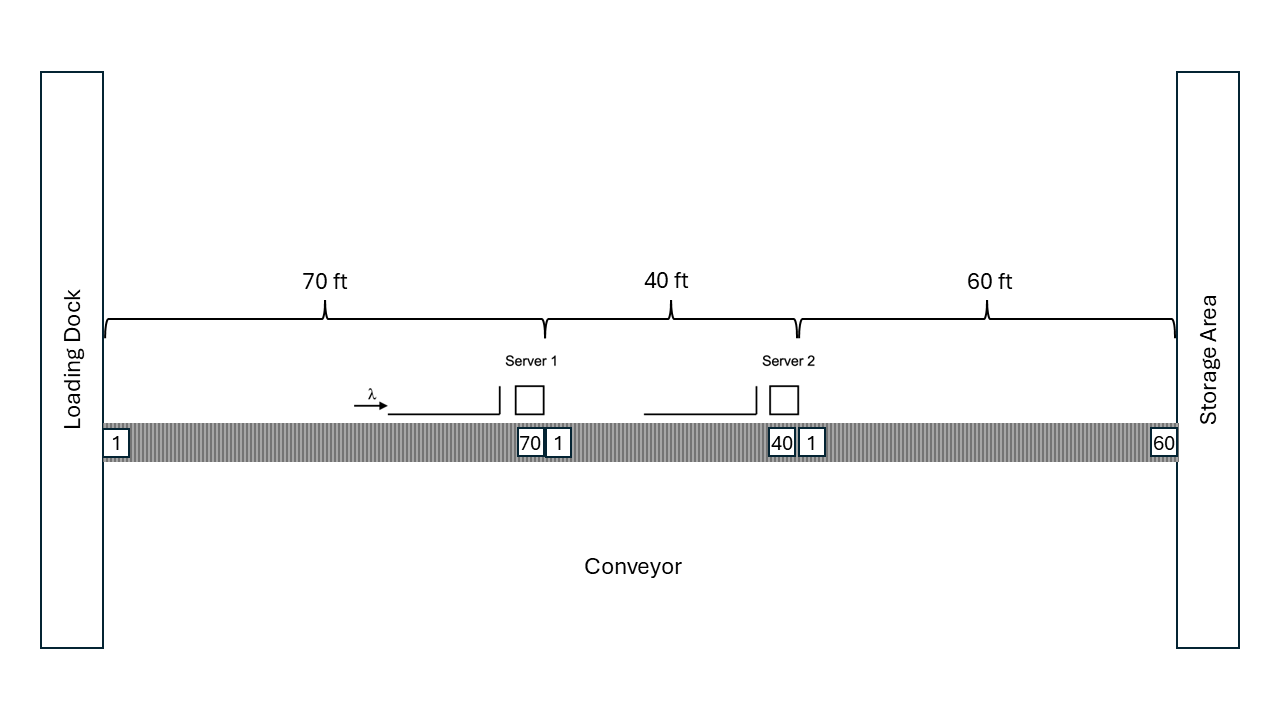
Figure 8.13: Tandem Queue with Conveyors
For this situation, we will assume that the conveyor speed is 30 feet per minute. There is one conveyor with three segments. The first segment will be 70 feet, the second segment will be 40 feet, and the third segment 60 feet. The beginning of the first segment starts at the loading dock and ends at the resource of the first station. The second segment starts at the end of the firs segment and goes to the resource of the second station. Finally, the third segment, goes from the resource at the second station to the store area. Initially, we will assume that the part is removed from the conveyor for the work to occur at the station. The time to remove the part from the conveyor and to place it back on the conveyor after processing is considered to be negligible.
We are going to show multiple models of this situation to compare and contrast different ways to model with conveyors.
- Model the system with simple delays acting as the conveyor.
- Model the system with the part exiting the conveyor for processing at each station using both accumulating and non-accumulating conveyors.
- Model the system with the part staying on the conveyor for processing at each station using both accumulating and non-accumulating conveyors.
8.4.2.1 Tandem Queue System with Conveyors and Deterministic Delays
To model the system with simple delays to represent the conveyor, we can use deterministic delays to represent the time to travel on the conveyor from location to location.
    private inner class Part : Entity() {
        val tandemQProcess: KSLProcess = process(isDefaultProcess = true) {
            wip.increment()
            timeStamp = time
            delay(delayDuration = 70.0/30.0) // 30 fpm for 70 ft
            use(resource = worker1, delayDuration = st1)
            delay(delayDuration = 40.0/30.0) // 30 fpm for 40 ft
            use(resource = worker2, delayDuration = st2)
            delay(delayDuration = 60.0/30.0) // 30 fpm for 60 ft
            timeInSystem.value = time - timeStamp
            wip.decrement()
        }
    }
Using a simple deterministic delay works reasonably well to represent the time of the part in the system. This approximation is reasonable if we do not care about the utilization of the conveyor in terms of space. Because the delay is deterministic, the sequence of parts that enter the conveyor is the same that exits at the stations. The results are useful for a baseline for more detailed modeling.
Conveyor via Deterministic Delay: Statistical Summary Report
| Name | Count | Average | Half-Width |
|---|---|---|---|
| worker1:InstantaneousUtil | 30 | 0.698 | 0.002 |
| worker1:NumBusyUnits | 30 | 0.698 | 0.002 |
| worker1:ScheduledUtil | 30 | 0.698 | 0.002 |
| worker1:Q:NumInQ | 30 | 1.598 | 0.037 |
| worker1:Q:TimeInQ | 30 | 1.6 | 0.035 |
| worker1:WIP | 30 | 2.296 | 0.039 |
| worker2:InstantaneousUtil | 30 | 0.901 | 0.004 |
| worker2:NumBusyUnits | 30 | 0.901 | 0.004 |
| worker2:ScheduledUtil | 30 | 0.901 | 0.004 |
| worker2:Q:NumInQ | 30 | 7.791 | 0.454 |
| worker2:Q:TimeInQ | 30 | 7.795 | 0.44 |
| worker2:WIP | 30 | 8.692 | 0.457 |
| TandemQueueWithConveyor:NumInSystem | 30 | 16.648 | 0.474 |
| TandemQueueWithConveyor:TimeInSystem | 30 | 16.662 | 0.444 |
| worker1:SeizeCount | 30 | 14982.233 | 40.422 |
| worker2:SeizeCount | 30 | 14978.633 | 40.03 |
8.4.2.2 Tandem Queue System with Conveyors Work Performed Off the Conveyor
Now, we will model the system using accumulating and non-accumulating conveyors and have the parts exit the conveyor and request the conveyor at each location. Let’s start by defining the conveyor. The basic tandem queueing system was modified to define the locations and conveyor with its segments.
class TandemQueueWithConveyors(
    parent: ModelElement,
    conveyorType: Conveyor.Type = Conveyor.Type.NON_ACCUMULATING,
    name: String? = null
) : ProcessModel(parent, name) {

    private val enter = "Enter"
    private val station1 = "Station1"
    private val station2 = "Station2"
    private val exit = "Exit"

    // velocity is in feet per min
    private val conveyor = Conveyor.builder(this, "Conveyor")
        .conveyorType(conveyorType)
        .velocity(30.0)
        .cellSize(1)
        .maxCellsAllowed(1)
        .firstSegment(enter, station1, 70)
        .nextSegment(station2, 40)
        .nextSegment(exit, 60)
        .build()
The velocity of the conveyor is 30 feet per minute. The basic cell size is 1 unit and the maximum number of cells that any part can occupy is one. The conveyor has three segments of 70, 40, and 60 feet, respectively. The conveyorType will be specified as accumulating or non-accumulating. The process description is a straight-forward use of the previously mentioned conveyor suspending functions.
    private inner class Part : Entity() {
        val tandemQProcess: KSLProcess = process(isDefaultProcess = true) {
            wip.increment()
            timeStamp = time
            val conveyorRequest = requestConveyor(conveyor = conveyor, entryLocation = enter, numCellsNeeded = 1)
            rideConveyor(conveyorRequest = conveyorRequest, destination = station1)
            exitConveyor(conveyorRequest)
            use(resource = worker1, delayDuration = st1)
            val conveyorRequest2 = requestConveyor(conveyor = conveyor, entryLocation = station1, numCellsNeeded = 1)
            rideConveyor(conveyorRequest = conveyorRequest2, destination = station2)
            exitConveyor(conveyorRequest = conveyorRequest2)
            use(resource = worker2, delayDuration = st2)
            val conveyorRequest3 = requestConveyor(conveyor = conveyor, entryLocation = station2, numCellsNeeded = 1)
            rideConveyor(conveyorRequest = conveyorRequest3, destination = exit)
            exitConveyor(conveyorRequest = conveyorRequest3)
            timeInSystem.value = time - timeStamp
            wip.decrement()
        }
    }
Notice how the conveyor request is captured and used within the ride and exit functions. If there is no need to use the conveyor request instances, then by using the convey() function, this process description can be significantly shortened.
        val tandemQProcess: KSLProcess = process(isDefaultProcess = true) {
            wip.increment()
            timeStamp = time
            convey(conveyor = conveyor, entryLocation = enter, destination = station1)
            use(resource = worker1, delayDuration = st1)
            convey(conveyor = conveyor, entryLocation = station1, destination = station2)
            use(resource = worker2, delayDuration = st2)
            convey(conveyor = conveyor, entryLocation = station2, destination = exit)
            timeInSystem.value = time - timeStamp
            wip.decrement()
        }
To specify that the conveyor is non-accumulating use Conveyor.Type.NON_ACCUMULATING and for accumulating use Conveyor.Type.ACCUMULATING when constructing the conveyor. The results for the non-accumulating case are as follows.
Non-Accumulating Working Off Conveyor: Statistical Summary Report
| Name | Count | Average | Half-Width |
|---|---|---|---|
| Conveyor:Enter:AccessQ:NumInQ | 30 | 0.001 | 0 |
| Conveyor:Enter:AccessQ:TimeInQ | 30 | 0.001 | 0 |
| Conveyor:Station1:AccessQ:NumInQ | 30 | 0.001 | 0 |
| Conveyor:Station1:AccessQ:TimeInQ | 30 | 0.001 | 0 |
| Conveyor:Station2:AccessQ:NumInQ | 30 | 0.001 | 0 |
| Conveyor:Station2:AccessQ:TimeInQ | 30 | 0.001 | 0 |
| Conveyor:Enter->Station1:NumOccupiedCells | 30 | 2.442 | 0.007 |
| Conveyor:Enter->Station1:CellUtilization | 30 | 0.035 | 0 |
| Conveyor:Station1->Station2:NumOccupiedCells | 30 | 1.395 | 0.004 |
| Conveyor:Station1->Station2:CellUtilization | 30 | 0.035 | 0 |
| Conveyor:Station2->Exit:NumOccupiedCells | 30 | 2.092 | 0.006 |
| Conveyor:Station2->Exit:CellUtilization | 30 | 0.035 | 0 |
| Conveyor:NumOccupiedCells | 30 | 5.929 | 0.017 |
| Conveyor:CellUtilization | 30 | 0.035 | 0 |
| worker1:InstantaneousUtil | 30 | 0.698 | 0.002 |
| worker1:NumBusyUnits | 30 | 0.698 | 0.002 |
| worker1:ScheduledUtil | 30 | 0.698 | 0.002 |
| worker1:Q:NumInQ | 30 | 1.611 | 0.037 |
| worker1:Q:TimeInQ | 30 | 1.613 | 0.036 |
| worker1:WIP | 30 | 2.309 | 0.039 |
| worker2:InstantaneousUtil | 30 | 0.901 | 0.004 |
| worker2:NumBusyUnits | 30 | 0.901 | 0.004 |
| worker2:ScheduledUtil | 30 | 0.901 | 0.004 |
| worker2:Q:NumInQ | 30 | 7.803 | 0.454 |
| worker2:Q:TimeInQ | 30 | 7.806 | 0.44 |
| worker2:WIP | 30 | 8.704 | 0.457 |
| TandemQueueWithConveyor:NumInSystem | 30 | 17.049 | 0.475 |
| TandemQueueWithConveyor:TimeInSystem | 30 | 17.064 | 0.444 |
| worker1:SeizeCount | 30 | 14982.133 | 40.487 |
| worker2:SeizeCount | 30 | 14978.7 | 40.085 |
The first thing to notice is that there are automatic statistics reported for the queues associated with the entry points of the conveyor. In addition, statistics are reported for the number of occupied cells and utilization of the cells for each segment. Finally, the conveyor’s overall cell utilization and number of occupied cells is reported. The results reported here are not very interesting. We see little waiting to get on the conveyor at the enter, station 1, and station 2 entry points. The utilization of the workers and queueing at the stations is almost the same as in the previous results. We notice that the time spent in the system is about 1 minute higher. This is likely due to the time to go through the cells to enter and exit the conveyor segments.
The same model can be executed with an accumulating conveyor by changing the conveyor type property of the conveyor. The results are presented here.
Accumulating Working Off the Conveyor: Statistical Summary Report
| Name | Count | Average | Half-Width |
|---|---|---|---|
| Conveyor:Enter:AccessQ:NumInQ | 30 | 0.001 | 0 |
| Conveyor:Enter:AccessQ:TimeInQ | 30 | 0.001 | 0 |
| Conveyor:Station1:AccessQ:NumInQ | 30 | 0.001 | 0 |
| Conveyor:Station1:AccessQ:TimeInQ | 30 | 0.001 | 0 |
| Conveyor:Station2:AccessQ:NumInQ | 30 | 0.001 | 0 |
| Conveyor:Station2:AccessQ:TimeInQ | 30 | 0.001 | 0 |
| Conveyor:Enter->Station1:NumOccupiedCells | 30 | 2.331 | 0.006 |
| Conveyor:Enter->Station1:CellUtilization | 30 | 0.033 | 0 |
| Conveyor:Station1->Station2:NumOccupiedCells | 30 | 1.332 | 0.004 |
| Conveyor:Station1->Station2:CellUtilization | 30 | 0.033 | 0 |
| Conveyor:Station2->Exit:NumOccupiedCells | 30 | 1.997 | 0.005 |
| Conveyor:Station2->Exit:CellUtilization | 30 | 0.033 | 0 |
| Conveyor:NumOccupiedCells | 30 | 5.659 | 0.015 |
| Conveyor:CellUtilization | 30 | 0.033 | 0 |
| worker1:InstantaneousUtil | 30 | 0.698 | 0.002 |
| worker1:NumBusyUnits | 30 | 0.698 | 0.002 |
| worker1:ScheduledUtil | 30 | 0.698 | 0.002 |
| worker1:Q:NumInQ | 30 | 1.596 | 0.037 |
| worker1:Q:TimeInQ | 30 | 1.598 | 0.035 |
| worker1:WIP | 30 | 2.294 | 0.039 |
| worker2:InstantaneousUtil | 30 | 0.901 | 0.004 |
| worker2:NumBusyUnits | 30 | 0.901 | 0.004 |
| worker2:ScheduledUtil | 30 | 0.901 | 0.004 |
| worker2:Q:NumInQ | 30 | 7.789 | 0.454 |
| worker2:Q:TimeInQ | 30 | 7.793 | 0.44 |
| worker2:WIP | 30 | 8.691 | 0.457 |
| TandemQueueWithConveyor:NumInSystem | 30 | 16.7 | 0.474 |
| TandemQueueWithConveyor:TimeInSystem | 30 | 16.714 | 0.444 |
| worker1:SeizeCount | 30 | 14982.2 | 40.432 |
| worker2:SeizeCount | 30 | 14978.6 | 40.033 |
The results for the accumulating conveyor case are a little better than for the non-accumulating conveyor. This is due to the fact that the conveyor continues to be engaged when allowing parts to enter and exit. The total time in the system is not statistically different from the deterministic delay case.
8.4.2.3 Tandem Queue System with Conveyors Work Performed On the Conveyor
In many systems, the work associated with a station can often be performed while the part is on the conveyor. As we will see, more care is needed in synchronizing the movement on the conveyor with the work content. This section illustrates how to change the process when the work is performed on the conveyor. Figure 8.14 illustrates that the worker is working on the part while it is on the last cells of the segments (cell 70 of segment 1 and cell 40 of segment 2).

Figure 8.14: Tandem Queue with Conveyors
To model this situation, we simply do not exit the conveyor at each station. The configuration of the conveyor remains the same. Notice that in the following code, we request the conveyor and ride it between the stations. Finally, we only exit the conveyor at the storage location (exit).
    private inner class Part : Entity() {
        val tandemQProcess: KSLProcess = process(isDefaultProcess = true) {
            wip.increment()
            timeStamp = time
            val conveyorRequest = requestConveyor(conveyor = conveyor, entryLocation = enter, numCellsNeeded = 1)
            rideConveyor(conveyorRequest = conveyorRequest, destination = station1)
            use(resource = worker1, delayDuration = st1)
            rideConveyor(conveyorRequest = conveyorRequest, destination = station2)
            use(resource = worker2, delayDuration = st2)
            rideConveyor(conveyorRequest = conveyorRequest, destination = exit)
            exitConveyor(conveyorRequest = conveyorRequest)
            timeInSystem.value = time - timeStamp
            wip.decrement()
        }
    }
Also, notice that we cannot use the convey() function because it assumes that the exit() function is used for each conveyance. The rideConveyor() function causes the conveyor to block until it is called again or until the exit() function is called. Thus, the use() functions are conceptually happening while the part is still on the conveyor. During this time, for an accumulating conveyor, the parts will pile up behind the blockage, essentially queueing up on the conveyor. Recall the analogy of the seriously deranged simulation professor in the airport. As we can see from the following results, working on the conveyor has some interesting effects on the statistics.
Accumulating Conveyor with Work On Conveyor: Statistical Summary Report
| Name | Count | Average | Half-Width |
|---|---|---|---|
| Conveyor:Enter:AccessQ:NumInQ | 30 | 0.001 | 0 |
| Conveyor:Enter:AccessQ:TimeInQ | 30 | 0.001 | 0 |
| Conveyor:Station1:AccessQ:NumInQ | 30 | 0 | 0 |
| Conveyor:Station1:AccessQ:TimeInQ | 0 | NaN | NaN |
| Conveyor:Station2:AccessQ:NumInQ | 30 | 0 | 0 |
| Conveyor:Station2:AccessQ:TimeInQ | 0 | NaN | NaN |
| Conveyor:Enter->Station1:NumOccupiedCells | 30 | 4.952 | 0.118 |
| Conveyor:Enter->Station1:CellUtilization | 30 | 0.071 | 0.002 |
| Conveyor:Station1->Station2:NumOccupiedCells | 30 | 11.418 | 0.549 |
| Conveyor:Station1->Station2:CellUtilization | 30 | 0.285 | 0.014 |
| Conveyor:Station2->Exit:NumOccupiedCells | 30 | 1.997 | 0.005 |
| Conveyor:Station2->Exit:CellUtilization | 30 | 0.033 | 0 |
| Conveyor:NumOccupiedCells | 30 | 18.367 | 0.643 |
| Conveyor:CellUtilization | 30 | 0.108 | 0.004 |
| worker1:InstantaneousUtil | 30 | 0.698 | 0.002 |
| worker1:NumBusyUnits | 30 | 0.698 | 0.002 |
| worker1:ScheduledUtil | 30 | 0.698 | 0.002 |
| worker1:Q:NumInQ | 30 | 0 | 0 |
| worker1:Q:TimeInQ | 30 | 0 | 0 |
| worker1:WIP | 30 | 0.698 | 0.002 |
| worker2:InstantaneousUtil | 30 | 0.901 | 0.004 |
| worker2:NumBusyUnits | 30 | 0.901 | 0.004 |
| worker2:ScheduledUtil | 30 | 0.901 | 0.004 |
| worker2:Q:NumInQ | 30 | 0 | 0 |
| worker2:Q:TimeInQ | 30 | 0 | 0 |
| worker2:WIP | 30 | 0.901 | 0.004 |
| TandemQueueWithConveyor:NumInSystem | 30 | 18.386 | 0.643 |
| TandemQueueWithConveyor:TimeInSystem | 30 | 18.401 | 0.61 |
| worker1:SeizeCount | 30 | 14982.167 | 40.405 |
| worker2:SeizeCount | 30 | 14977.633 | 40.149 |
Notice that the queues for the workers are zero. This is because the entity that seizes the worker blocks all the entities behind it on the conveyor. They never get a chance to seize the worker until the worker is available. Notice how the number of occupied cells mirrors the queue sizes from the previous results. Essentially, the entities are waiting on the conveyor. Notice also that the queues for entry onto the conveyor at station 1 and 2 are zero. This is because no parts exit at those stations and thereby need to wait to get back on the conveyor. The conveyor can be configured not to report these unnecessary statistics.
Now let’s see the effect of using a non-accumulating conveyor in the situation.
Non-accumulating Conveyor with Work On Conveyor:Statistical Summary Report
| Name | Count | Average | Half-Width |
|---|---|---|---|
| Conveyor:Enter:AccessQ:NumInQ | 30 | 2359.251 | 42.718 |
| Conveyor:Enter:AccessQ:TimeInQ | 30 | 2359.658 | 40.409 |
| Conveyor:Station1:AccessQ:NumInQ | 30 | 0 | 0 |
| Conveyor:Station1:AccessQ:TimeInQ | 0 | NaN | NaN |
| Conveyor:Station2:AccessQ:NumInQ | 30 | 0 | 0 |
| Conveyor:Station2:AccessQ:TimeInQ | 0 | NaN | NaN |
| Conveyor:Enter->Station1:NumOccupiedCells | 30 | 70 | 0 |
| Conveyor:Enter->Station1:CellUtilization | 30 | 1 | 0 |
| Conveyor:Station1->Station2:NumOccupiedCells | 30 | 40 | 0 |
| Conveyor:Station1->Station2:CellUtilization | 30 | 1 | 0 |
| Conveyor:Station2->Exit:NumOccupiedCells | 30 | 60 | 0 |
| Conveyor:Station2->Exit:CellUtilization | 30 | 1 | 0 |
| Conveyor:NumOccupiedCells | 30 | 170 | 0 |
| Conveyor:CellUtilization | 30 | 1 | 0 |
| worker1:InstantaneousUtil | 30 | 0.564 | 0.002 |
| worker1:NumBusyUnits | 30 | 0.564 | 0.002 |
| worker1:ScheduledUtil | 30 | 0.564 | 0.002 |
| worker1:Q:NumInQ | 30 | 0 | 0 |
| worker1:Q:TimeInQ | 30 | 0 | 0 |
| worker1:WIP | 30 | 0.564 | 0.002 |
| worker2:InstantaneousUtil | 30 | 0.728 | 0.001 |
| worker2:NumBusyUnits | 30 | 0.728 | 0.001 |
| worker2:ScheduledUtil | 30 | 0.728 | 0.001 |
| worker2:Q:NumInQ | 30 | 0 | 0 |
| worker2:Q:TimeInQ | 30 | 0 | 0 |
| worker2:WIP | 30 | 0.728 | 0.001 |
| TandemQueueWithConveyor:NumInSystem | 30 | 2530.251 | 42.718 |
| TandemQueueWithConveyor:TimeInSystem | 30 | 2530.917 | 40.085 |
| worker1:SeizeCount | 30 | 12081.5 | 31.211 |
| worker2:SeizeCount | 30 | 12081.5 | 31.211 |
These results are dramatically different. Why? We again see that the queues for the resources are zero; however, the queue for accessing the conveyor at the enter location is out of control. Why might this be the expected behavior? Recall that for a non-accumulating conveyor, the segments disengage when a part is entering or has reached its destination. The rideConveyor() function moves the part to its destination on the conveyor. When the part reaches its destination, the conveyor disengages again. The cell that the part occupies on the conveyor remains occupied while the part is being processed. Thus, when the part is using the worker at station 1 (or station 2) the conveyor is essentially stopped. No parts are moving on the conveyor. Therefore, the parts trying to enter at the beginning of the conveyor must wait for the service of every part on their segment of the conveyor. This results in a huge bottleneck. Obviously, this is not how we would design such a system. The specification of a non-accumulating conveyor is not appropriate for this situation; however, the usage of an accumulating conveyor is very appropriate. It may be possible to use non-accumulating conveyors when the work is performed on the conveyor; however, the work needs to be perfectly balanced. In the next section, we will see how to model the test and repair system with a circular conveyor.
8.4.3 Test and Repair via Conveyors
For simplicity, the test and repair shop will be used for illustrating the use of conveyors. Figure 8.15 shows the test and repair shop with the conveyors and the distance between the stations. From the figure, the distances from each station going in clockwise order are as follows:
Diagnostic station to test station 1, 20 feet
Test station 1 to test station 2, 20 feet
Test station 2 to repair, 15 feet
Repair to test station 3, 45 feet
Test station 3 to diagnostics, 30 feet

Figure 8.15: Test and repair shop with conveyors
Assume that the conveyor’s velocity is 10 feet per minute. These figures have been provided in this example; however, in modeling a real system, you will have to tabulate this information. To illustrate the use of entity sizes, assume the following concerning the parts following the four test plans:
Test plan 1 and 2 parts require 1 foot of space while riding on the conveyor
Test plan 3 and 4 parts require 2 feet of space while riding on the conveyor
For this example, we will assume that the conveyor is an accumulating conveyor. Now, we are ready to define the conveyor and its segments.
8.4.3.1 Test and Repair Conveyor Definitions
To define the conveyor within code, we can use the builder functionality provided by the Conveyor class’s companion object. Because we have parts that require different amounts of space on the conveyor, we need to set the maximum number of cells allowed by any entity. The following KSL code provides the conveyor definition. Also, note the the code turns off the reporting of access queues associated with the repair station. This is done because no parts need to access the conveyor at the repair station. For this illustrative example, the code also prints out the conveyor configuration, which we will review.
    private val loopConveyor: Conveyor = Conveyor.builder(this, "LoopConveyor")
        .conveyorType(Conveyor.Type.ACCUMULATING)
        .velocity(10.0)
        .cellSize(1)
        .maxCellsAllowed(2)
        .firstSegment(myDiagnostics.name, myTest1.name, 20)
        .nextSegment(myTest2.name, 20)
        .nextSegment(myRepair.name, 15)
        .nextSegment(myTest3.name, 45)
        .nextSegment(myDiagnostics.name, 30)
        .build()

    init {
        loopConveyor.accessQueueAt(myRepair.name).defaultReportingOption = false
        println(loopConveyor)
    }
The configuration of the conveyor can be seen via its toString() function. As we can see from the output, we have an accumulating conveyor with a velocity of 10 feet per minute. The total length of the conveyor is 130 feet. Since each cell equates to 1 foot, there are 130 cells. There are five segments. Since the conveyor’s last location is the same as its first location, it is considered a circular conveyor. The conveyor also determines which locations are downstream, relative to the first location. This ensures that the movement request from one location to another location is feasible relative to the path defined by the conveyor. As noted, the segments consist of a sequence of cells. For example, the first segment is between diagnostics and the test 1 station. The entry location for diagnostics is cell 1 and the exit location for test 1 is cell 20. Note that every location has both an entry cell and an exit cell.
Conveyor : LoopConveyor
type = ACCUMULATING
is circular = true
velocity = 10.0
cellSize = 1
max number cells allowed to occupy = 2
cell Travel Time = 0.1
Segments:
first location = Diagnostics
last location = Diagnostics
Segment: 1 = (start = Diagnostics --> end = Test1 : length = 20)
Segment: 2 = (start = Test1 --> end = Test2 : length = 20)
Segment: 3 = (start = Test2 --> end = Repair : length = 15)
Segment: 4 = (start = Repair --> end = Test3 : length = 45)
Segment: 5 = (start = Test3 --> end = Diagnostics : length = 30)
total length = 130
Downstream locations:
Diagnostics : [Test1 -> Test2 -> Repair -> Test3 -> Diagnostics]
Test1 : [Test2 -> Repair -> Test3 -> Diagnostics]
Test2 : [Repair -> Test3 -> Diagnostics]
Repair : [Test3 -> Diagnostics]
Test3 : [Diagnostics]
Segment Cells:
Locations[Diagnostics->Test1] = Cells[1..20]
Locations[Test1->Test2] = Cells[21..40]
Locations[Test2->Repair] = Cells[41..55]
Locations[Repair->Test3] = Cells[56..100]
Locations[Test3->Diagnostics] = Cells[101..130]
Now, we are ready to update the process description for the test and repair system to use the conveyor.
8.4.3.2 Test and Repair Conveyor Processing
The test plans for the problem remain the same as in the previous examples; however, the parts that follow different test plans require different cell sizes. To facilitate the specification of cell size requirements for each test plan, we can use a map to hold the requirements.
We can use the cellSizes map to determine the number of cells need by the part when using the conveyor. By using the convey() function, the process description becomes very compact.
    private inner class Part : Entity() {

        // determine the test plan
        val plan: List<TestPlanStep> = planList.randomElement
        val cellsNeeded = cellSizes[plan]!!

        val testAndRepairProcess: KSLProcess = process(isDefaultProcess = true) {
            wip.increment()
            timeStamp = time
            //every part goes to diagnostics
            use(resource = myDiagnostics, delayDuration = diagnosticTime)
            // get the iterator
            val itr = plan.iterator()
            // iterate through the plan
            var entryLocation = myDiagnostics.name
            while (itr.hasNext()) {
                val tp = itr.next()
                convey(
                    conveyor = loopConveyor,
                    entryLocation = entryLocation,
                    destination = tp.resource.name,
                    numCellsNeeded = cellsNeeded
                )
                use(resource = tp.resource, delayDuration = tp.processTime)
                entryLocation = tp.resource.name
            }
            timeInSystem.value = time - timeStamp
            wip.decrement()
        }
    }
When a part is created, its test plan is randomly determined and assigned. Then, the cellSizes map is used to look up the assigned number of cells needed when riding on the conveyor. The main challenge associated with the process code is ensuring that the entry location is correctly specified when using the conveyor. Note that before the iterator loop, we specify the entry location, essentially as the station that we are leaving. This is the location that we need to access to get on the conveyor. This variable is updated again after using the resource. It may seem strange to specify the location via the stored references of the resources to visit. However, since the locations associated with a conveyor need only be instances of classes that implement the IdentityIfc interface, and all model elements implement this interface, model elements such as resources can be used as locations via the model element’s name property.
The results of executing the model for 30 replications of 20,000 time units (minutes) with a warm up period of 5000 minutes is as follows.
Statistical Summary Report
| Name | Count | Average | Half-Width |
|---|---|---|---|
| Diagnostics:InstantaneousUtil | 10 | 0.753 | 0.007 |
| Diagnostics:NumBusyUnits | 10 | 1.506 | 0.014 |
| Diagnostics:ScheduledUtil | 10 | 0.753 | 0.007 |
| Diagnostics:Q:NumInQ | 10 | 2.006 | 0.129 |
| Diagnostics:Q:TimeInQ | 10 | 39.92 | 2.475 |
| Diagnostics:WIP | 10 | 3.512 | 0.142 |
| Test1:InstantaneousUtil | 10 | 0.858 | 0.007 |
| Test1:NumBusyUnits | 10 | 0.858 | 0.007 |
| Test1:ScheduledUtil | 10 | 0.858 | 0.007 |
| Test1:Q:NumInQ | 10 | 2.984 | 0.272 |
| Test1:Q:TimeInQ | 10 | 52.914 | 4.436 |
| Test1:WIP | 10 | 3.842 | 0.279 |
| Test2:InstantaneousUtil | 10 | 0.781 | 0.006 |
| Test2:NumBusyUnits | 10 | 0.781 | 0.006 |
| Test2:ScheduledUtil | 10 | 0.781 | 0.006 |
| Test2:Q:NumInQ | 10 | 1.636 | 0.07 |
| Test2:Q:TimeInQ | 10 | 43.209 | 1.588 |
| Test2:WIP | 10 | 2.417 | 0.074 |
| Test3:InstantaneousUtil | 10 | 0.866 | 0.006 |
| Test3:NumBusyUnits | 10 | 0.866 | 0.006 |
| Test3:ScheduledUtil | 10 | 0.866 | 0.006 |
| Test3:Q:NumInQ | 10 | 2.611 | 0.19 |
| Test3:Q:TimeInQ | 10 | 51.966 | 3.554 |
| Test3:WIP | 10 | 3.478 | 0.194 |
| Repair:InstantaneousUtil | 10 | 0.872 | 0.004 |
| Repair:NumBusyUnits | 10 | 2.616 | 0.012 |
| Repair:ScheduledUtil | 10 | 0.872 | 0.004 |
| Repair:Q:NumInQ | 10 | 1.282 | 0.091 |
| Repair:Q:TimeInQ | 10 | 25.535 | 1.703 |
| Repair:WIP | 10 | 3.898 | 0.101 |
| TestAndRepairWithConveyor:NumInSystem | 10 | 18.263 | 0.541 |
| TestAndRepairWithConveyor:TimeInSystem | 10 | 363.6 | 8.921 |
| ProbWithinLimit | 10 | 0.802 | 0.018 |
| LoopConveyor:NumOccupiedCells | 10 | 1.667 | 0.01 |
| LoopConveyor:CellUtilization | 10 | 0.013 | 0 |
| Diagnostics:SeizeCount | 10 | 12540.1 | 71.465 |
| Test1:SeizeCount | 10 | 14057.6 | 116.559 |
| Test2:SeizeCount | 10 | 9442.7 | 63.431 |
| Test3:SeizeCount | 10 | 12532.4 | 70.688 |
| Repair:SeizeCount | 10 | 12526.6 | 69.078 |
The results produced by the KSL are within statistical variation of the same system modeled with a commercial simulation language discussed in this book.
8.4.4 Miscellaneous Concepts in Conveyor Modeling
This section presents some common conveyor modeling situations that can be modeled using the KSL: conveyors that merge, conveyors that diverge, and conveyors that recirculate.
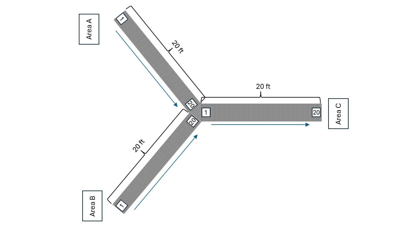
Figure 8.16: Two Conveyors Merge into One
Figure 8.16 illustrates the concept of merging. In the figure, there are three conveyors. The first conveyor goes from area A to the sorting area. The second conveyor goes from area B to the sorting area. The third conveyor goes from the sorting area to processing at area C. The most important aspect of modeling this situation is to note that there are three conveyors. Thus, there would be three instances of the KSL Conveyor class that need to be specified. Generally, the velocities of the conveyors may be the same, but not necessarily. To model this situation, we must be able to transfer an entity on one conveyor to another conveyor. The transferTo() suspending function provides this functionality.
The transferTo() suspending function causes the entity to transfer from its current conveyor to another conveyor. The entity will suspend while accessing the required cells at the next conveyor. Once the desired cells are obtained the entity will exit its current conveyor and be positioned to ride on the next conveyor. After executing this function, the entity will be blocking the entry cell of the next conveyor and must then execute the rideConveyor() function to move on the new conveyor. The transfer will include the time needed for the entity to move through the exit cells of the current conveyor, any waiting to access the next conveyor, and be positioned to ride on the next conveyor. There are some important conditions that must be met to utilize this function. First, the entity must be on a conveyor and located at an exit cell/location. Obviously, the entity must transfer to a different conveyor than the one that it currently occupies. Finally, the entity’s exit cell’s location must correspond to the same location on the conveyor to which it is transferring. That is, the location of transfer must be an exit location on the current conveyor and an entry location on the subsequent conveyor. In Figure 8.16, the cell denoted as 20 on the area A and B conveyors are exit cells. The cell denoted 1 on the conveyor heading towards area C is the entry cell. Parts ride the two input conveyors until they reach the end of the conveyor (cell 20) and then transfer to cell 1 of the subsequent conveyor.
The situation illustrated in Figure 8.16 can be modeled with code similar to the following. First we need to define the three conveyors.
class ConveyorMerging(
    parent: ModelElement,
    name: String? = null
) : ProcessModel(parent, name) {

    private val areaA = "AreaA"
    private val areaB = "AreaB"
    private val sorting = "Sorting"
    private val areaC = "AreaC"

    private val conveyor1 = Conveyor.builder(this, "Conveyor1")
        .conveyorType(Conveyor.Type.ACCUMULATING)
        .velocity(1.0)
        .cellSize(1)
        .maxCellsAllowed(1)
        .firstSegment(areaA, sorting, 20)
        .build()

    private val conveyor2 = Conveyor.builder(this, "Conveyor2")
        .conveyorType(Conveyor.Type.ACCUMULATING)
        .velocity(1.0)
        .cellSize(1)
        .maxCellsAllowed(1)
        .firstSegment(areaB, sorting, 20)
        .build()

    private val conveyor3 = Conveyor.builder(this, "Conveyor3")
        .conveyorType(Conveyor.Type.ACCUMULATING)
        .velocity(1.0)
        .cellSize(1)
        .maxCellsAllowed(1)
        .firstSegment(sorting, areaC, 20)
        .build()
Now, we can define processes for the entities that use the conveyors. There could be a variety of ways to handle this situation; however, for simplicity, we will assume that there are two types of entities, one coming from area 1 and the other coming from area 2. The process code for a part starting at area 1 would be something like this:
    private val tba1 = ExponentialRV(10.0, 1)
    private val generateAreaAParts = EntityGenerator(this::AreaAPart, tba1, tba1)

    private val tba2 = TriangularRV(10.0, 16.0, 18.0, 2)
    private val generateAreaBParts = EntityGenerator(this::AreaBPart, tba2, tba2)

    private val myAreaASystemTime = Response(this, "AreaASystemTime")
    private val myAreaBSystemTime = Response(this, "AreaBSystemTime")

    private inner class AreaAPart : Entity() {
        val mergeProcess: KSLProcess = process(isDefaultProcess = true) {
            val cr = requestConveyor(conveyor = conveyor1, entryLocation = areaA, numCellsNeeded = 1)
            rideConveyor(conveyorRequest = cr, destination = sorting)
            val tr = transferTo(conveyorRequest = cr, nextConveyor = conveyor3, entryLocation = sorting)
            rideConveyor(conveyorRequest = tr, destination = areaC)
            exitConveyor(conveyorRequest = tr)
            myAreaASystemTime.value = time - entity.createTime
        }
    }

    private inner class AreaBPart : Entity() {
        val mergeProcess: KSLProcess = process(isDefaultProcess = true) {
            val cr = requestConveyor(conveyor = conveyor2, entryLocation = areaB, numCellsNeeded = 1)
            rideConveyor(conveyorRequest = cr, destination = sorting)
            val tr = transferTo(conveyorRequest = cr, nextConveyor = conveyor3, entryLocation = sorting)
            rideConveyor(conveyorRequest = tr, destination = areaC)
            exitConveyor(conveyorRequest = tr)
            myAreaBSystemTime.value = time - entity.createTime
        }
    }
Notice that the part requests the cells on the conveyor at area A, and then rides to sorting. Then, the part transfers from conveyor 1 to conveyor 3. Notice that the returned conveyor request must be supplied to the transferTo() function. Also, notice that the sorting location is both an exit location for conveyor 1 and an entry location for conveyor 3. The transferTo() function returns a new conveyor request that represents the fact that the entity is now on the next conveyor. This new conveyor request is used to ride conveyor 3 to the processing at area C and to exit at the processing area. The logic for the parts travelling from area B to processing is very similar. They start at area B and transfer to conveyor 3 at the sorting area. It is important to note that the parts from the two feeder conveyors will compete for the entry cell of conveyor 3 at the sorting location. The parts traveling on conveyors 1 and 2 do not immediately exit at the transfer point. They first receive the necessary cells on conveyor 3 before exiting their current conveyor. Thus, they will block their current conveyor while waiting to access the next conveyor. Thus, we can see why it may be important to model this situation with accumulating conveyors.
Figure 8.17 also illustrates the concept of merging. In this case, there are two conveyors, with one conveyor connecting to the mid-point of the other conveyor. Again, the transferTo() function for use with conveyors can be used to address this situation.
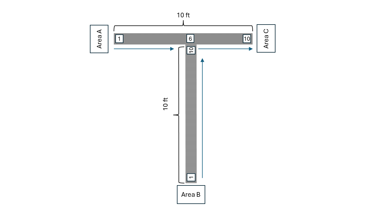
Figure 8.17: One Conveyor Merges into Another
The code for this situation would be very similar to the previous example. The important thing to note is that there are only two conveyors. The main conveyor has two segments. The feeder conveyor has one segment. The exit cell/location of the feeder conveyor matches the entry cell/location of the second segment of the main conveyor at cell 6. For example, the main conveyor goes from area A location to the midpoint location to the end point location, with lengths 5 feet respectively. The second conveyor is a single conveyor from the area B location to the midpoint location with a length of 10 feet. In other words, they share a common location positioned at cell 6.
The entities arrive at the area A and area B locations. Entities that arrive at
the area A location first convey to the midpoint location and then
immediately convey to the end point location They do not exit the
conveyor at the midpoint location. Entities from the area B location are
conveyed to the midpoint location. Once at the midpoint location they
first request cells from the main conveyor and then exit their conveyor. This would be modeled using the transferTo() function. This causes entities coming from area B to potentially wait for space on the main
conveyor. This basic idea can be expanded to any number of feeder conveyors along a longer main conveyor. The end of each feeder conveyor would be mapped to the entry cell of a segment along the main conveyor.
Figure 8.18 illustrates the concept of a diverging conveyor. This situation is the reverse Figure 8.16 with 3 conveyors. One conveyor from area A to sorting point, connects to two other conveyors, one conveyor from sorting to area B and the other conveyor from sorting to area C.
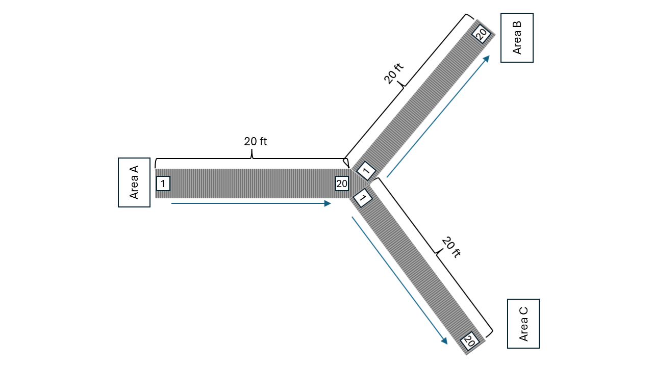
Figure 8.18: One Conveyor Diverges Into Two Conveyors
Diverging conveyors are often used in systems that sort items. The items come in on one main conveyor and are transferred to any number of other conveyors based on their attributes (e.g. destination). In this simple illustration, the parts arrive to the arrival area A and access a conveyor to the sorting area. Once an entity reaches the sorting station, the entity would need to determine which of the two conveyors to access. This could be easily accomplished with an if statement or other decision logic. Then the entity would transfer to the subsequent conveyor, ride and then exit. The exercises ask the reader to implement this situation.
With a little imagination a more sophisticated sorting location can be implemented. For example, a number of conveyors that handle the parts by destination might be used in the system. When the parts are created they
are given an attribute indicating their destination station. When they
get to the sorting location, a Kotlin when statement can be used to pick the
correct conveyor handling their destination.
The final conveyor modeling situation to be described is that of a recirculating conveyor. We saw in Section 8.4.3 for modeling the test and repair system, that we can create and use a circular conveyor. That is, a conveyor for which its ending location also corresponds to its entry location. A recirculating conveyor is a circular conveyor in which the entities may ride on the conveyor until there is adequate space at their desired location. In essence the conveyor is used as space to hold the entities that cannot get off due to inadequate space at the necessary station. For example, suppose that in the test and repair shop there was only space for one waiting part at test station two. Thus, the size of test station two’s queue can be at most 1. In such a situation, when a part designated for work at test station 2 reaches the location, it needs to check if the available space (queue at test station 2) is available. If there is space available in front of the testing machine, then the part can exit the conveyor. Now, what should we do if there is inadequate space at the test station?
We could wait on the conveyor at test station 2 until there is space, but this will block the entire conveyor while the processing at test station 2 proceeds and its queue reduces. Alternatively, we would not exit the conveyor at test station 2 and instead ride the full conveyor’s length back to test station 2. By the time that the entity has ridden around the conveyor, there may now be space available at test station 2. As previously noted, in essence, the entire conveyor is being used as waiting space. This kind of situation can be easily modeled with if statements that check if the there is space and if not cause the entity to continue riding. The exercises ask the reader to implement this situation.