10.9 Exercises
Exercise 10.1 Use an RSPLINE solver to solve the reorder point, reorder quantity problem discussed in the chapter. Compare its results to the results from Section 10.7.
Exercise 10.2 Use a simulated annealing solver for the reorder point, reorder quantity problem discussed in the chapter. Run a set of experiments to evaluate the effect of the initial temperature on the performance of the algorithm. Use different starting points to understand if their is an interaction between the starting point and the initial temperature in terms of execution time to achieve a solution.
Exercise 10.3 Suppose a manufacturing system contains 5 machines, each subject to randomly occurring breakdowns. A machine runs for an amount of time that is an exponential random variable with a mean of 10 hours before breaking down. At present there are 2 operators to fix the broken machines. The amount of time that an operator takes to service the machines is exponential with a mean of 4 hours. An operator repairs only 1 machine at a time. If more machines are broken down than the current number of operators, the machines must wait for the next available operator for repair. They form a FIFO queue to wait for the next available operator. The number of operators required to tend to the machines in order to minimize down time in a cost effective manner is desired. Assume that it costs the system 60 dollars per hour for each machine that is broken down. Each operator is paid 15 dollars per hour regardless of whether they are repairing a machine or not.
- Formulate an optimization problem that minimizes the total expected cost per hour of operating this system in terms of the number operators.
- Build a discrete-event dynamic simulation model to estimate the total expected cost per hour as a function of the number of operators.
- Apply a simulated annealing solver to find the optimal number of operators to this problem. How confident are you in your result?
- Did you need simulation optimization to solve this problem?
Exercise 10.4 Consider Exercise 7.13 of Chapter 7. After building a simulation model for the situation, apply the following solvers to find the optimal reorder point and reorder quantity that minimizes the total cost in terms of ordering, holding, and back order costs.
- Stochastic hill climbing
- Cross entropy
- Simulated annealing
- RSPLINE
Compare the performance of the solvers in terms of execution time, number of oracle calls, number of replications, and solution quality.
Exercise 10.5 A key issue for the simulated annealing algorithm is the specification of the initial temperature. An approach to determining a good initial temperature is discussed in this stack exchange discussion which references (Ben-Ameur 2004). Read the paper and implement a function that will provide a default initial temperature for the simulated annealing solver.
Exercise 10.6 Consider the application of the cross-entropy solver to the reorder point, reorder quantity inventory problem in Section 10.7.1. Run the solver with and without using a solution cache. Compare the performance of the cases in terms of execution time, number of oracle calls, number of replications, and solution quality.
Exercise 10.7 In a continuous review (s, S) inventory control system, the system operates essentially the same as an (r, Q) control policy except that when the reorder point, s, is reached, the system instead orders enough inventory to reach a maximum inventory level of S. Thus, the amount of the order will vary with each order. Repeat the analysis of Exercise 10.4 assuming that the SKU is controlled with a (s, S) policy. Assume that s = 4 and S = 7.
Exercise 10.8 Consider a shop that produces and stocks items. The items are produced in lots. The demand process for each item is Poisson with the rate given below. Back ordering is permitted. The pertinent data for each of the items is given in the following table. The carrying charge on each item is 0.20. The lead time is considered constant with the value provided in the table. Assume that there are 360 days in each year.
| Item | 1 | 2 | 3 | 4 | 5 | 6 |
| Demand Rate (units per year) | 1000 | 500 | 2000 | 100 | 50 | 250 |
| Unit cost (dollars per unit) | 20 | 100 | 50 | 500 | 1000 | 200 |
| Lead time mean (days) | 2 | 5 | 5 | 6 | 14 | 8 |
Suppose that management desires to set the optimal (r, Q) policy variables for each of the items so as to minimize the total holding cost and ordering costs. Assume that it costs approximately $5 to prepare and process each order. In addition, they desire to have the system fill rate to be no lower than 80% and no individual item’s fill rate to be below 60%. They also desire to have the average customer wait time (for any part) to be less than or equal to 3 days. Simulate this system and use simulation optimization to find an optimal policy recommendation for the items. You might start by analyzing the parts individually to have initial starting values for the optimization search.
Exercise 10.9 As illustrated in Figure 10.28, a multi-echelon system consists of an external supplier, a warehouse, and a set of retailers. Assume that there is only 1 item type stocked at each location within the system. The warehouse supplies each of the four retailers when they make a replenishment request.
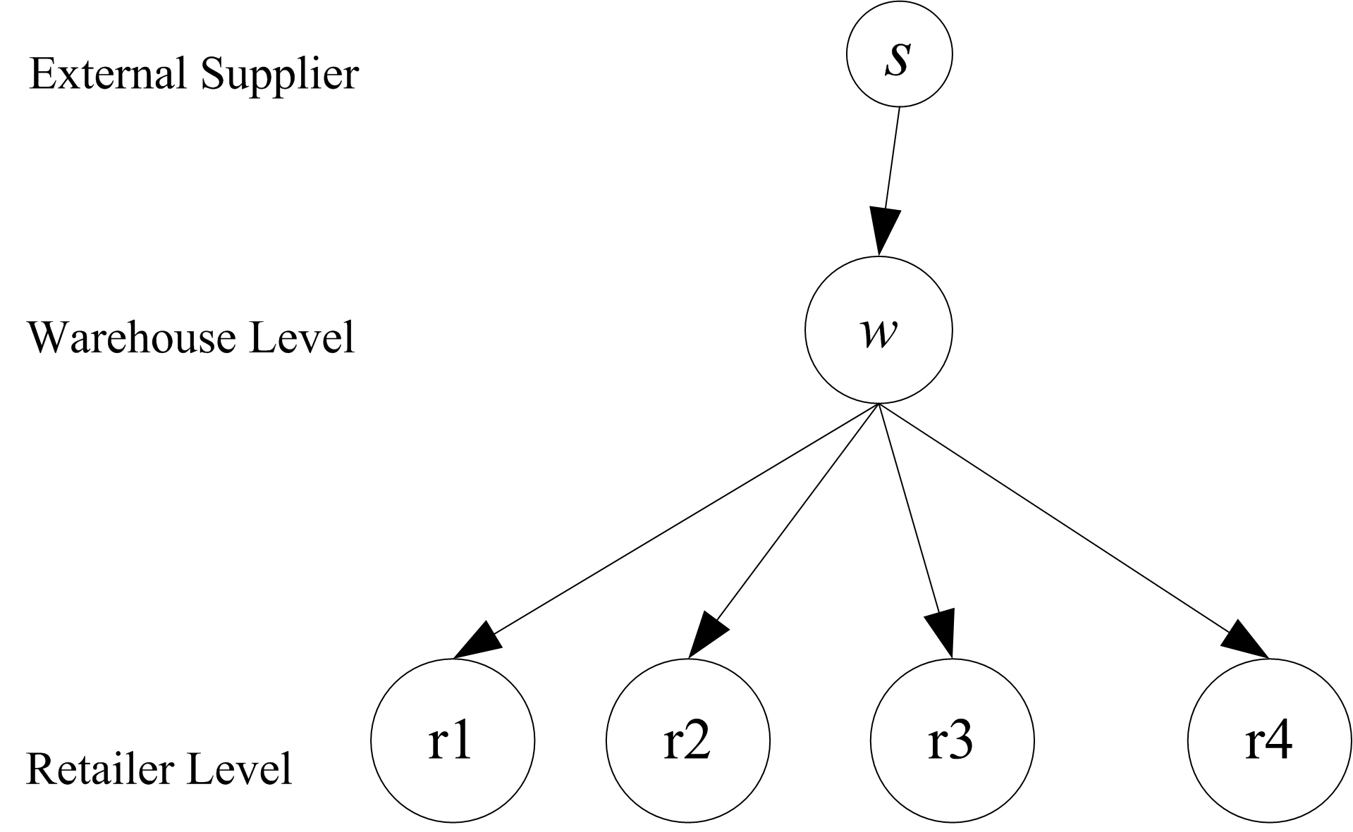
Figure 10.28: Multi-Echelon Inventory System
Suppose that the retail locations do not allow back ordering. That is, customers who arrive when there is not enough to fill their demand are lost. In addition, suppose that the amount demanded for each customer is governed by a shifted geometric random variable with parameter p = 0.9. The warehouse and the retailers control the SKU with (s, S) policies as shown in the following table.
| Policy (s, S) | Demand Poisson (mean rate per day) | |
|---|---|---|
| Retailer 1 | (1, 3) | (0.2) |
| Retailer 2 | (1, 5) | (0.1) |
| Retailer 3 | (2, 6) | (0.3) |
| Retailer 4 | (1, 4) | (0.4) |
| Warehouse | (4, 16) |
The overall rate to the retailers is 1 demand per day, but individually they experience the rates as shown in the table. In other words, the retailers are not identical in terms of the policy or the demand that they experience. The lead time is 5 days for the warehouse and 1 day for each retailer. The warehouse allows back ordering.
- Develop an KSL model for this situation. Estimate the expected number of lost sales per year for each retailer, the average amount of inventory on hand at the retailers and at the warehouse, the fill rate for each retailer and for the warehouse, and the average number of items back ordered at the warehouse. Run the model for 10 replications of 3960 days with a warm up of 360 days.
- The unit cost of the item is 10 dollars and the holding charge at each retailer is (10, 15, 20, 25) percent per unit per year for the four retailers, respectively. Suppose the the holding charge at the warehouse is 15 percent per unit per year. Assume that the ordering cost at each location is approximately 2 dollars for each order placed. Develop an optimization model that will determine the optimal inventory policy parameters for each location that minimizes the overall total cost of inventory ordering and holding costs subject to at least 96 percent fill rates at each of the retailer locations and at least a 90 percent fill rate at the warehouse.