10.5 Characterizing Simulation Optimization Algorithms

The KSL ksl.simopt.solvers package provides a general framework for designing and implementing simulation optimization algorithms. For the purpose of this section, we call these algorithms, solvers. The solver package provides the Solver abstract base class that can be specialized to implement different algorithms. The KSL also provides a set of implemented algorithms for use on simulation optimization problems. Figure 10.21 illustrates the class hierarchy for existing solvers. The Solver class and the StochasticSolver classes are abstract base classes. Essentially, the Solver class defines the basic properties and methods needed for solving an optimization problem. The StochasticSolver class assumes that the optimization process may incorporate random search and provides the solver access to random streams.

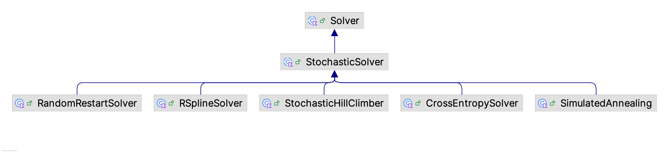
Figure 10.21: The Solver Class Hierarchy

The constructors for the Solver class and the StochasticSolver class show that a solver must have a reference to the problem and an evaluator. In addition, solvers are conceptualized as iterative processes. Each iteration of a solver may evaluate solutions and move towards a “best” solution. Thus, solvers require a limit on the maximum number of iterations. As we will see, there will be more general ways to implement stopping conditions; however, every solver has a pre-specified maximum number of iterations permitted before it will stop.

Within the context of simulation optimization, the supplied evaluator promises to execute requests for evaluations of the simulation model at particular design points (as determined by the algorithm). In addition, because of the stochastic nature of the evaluation, the solver may request one or more replications for its evaluation requests. The number of replications may change dynamically, and thus the user needs to supply a function to determine the number of replications per evaluation. Within the framework of the hooks for sub-classes, the user could specify more complex procedures for determining the number of replications per evaluation. The constructor provides a the ReplicationPerEvaluationIfc interface to specify the current number of replications for each evaluation request. The number of replications can vary as the solver proceeds. Solvers also emit solutions to permit tracking/tracing the solution process.

abstract class Solver(
    val problemDefinition: ProblemDefinition,
    evaluator: EvaluatorIfc,
    maximumIterations: Int,
    var replicationsPerEvaluation: ReplicationPerEvaluationIfc,
    name: String? = null
) : IdentityIfc by Identity(name), Comparator<Solution>, SolverEmitterIfc by SolverEmitter() {

The StochasticSolver inherits from the Solver class and requires that a source of random streams be provided. It also allows stream control.

abstract class StochasticSolver(
    problemDefinition: ProblemDefinition,
    evaluator: EvaluatorIfc,
    maxIterations: Int,
    replicationsPerEvaluation: ReplicationPerEvaluationIfc,
    streamNum: Int = 0,
    val streamProvider: RNStreamProviderIfc = KSLRandom.DefaultRNStreamProvider,
    name: String? = null
) : Solver(problemDefinition, evaluator, maxIterations, replicationsPerEvaluation, name), RNStreamControlIfc {

10.5.1 Structure of the Iterative Process

A solver is an iterative algorithm that searches for the optimal solution for a defined problem. In the abstract Solver class, the algorithm is conceptualized as having a main iterative loop. The basic algorithm is structured conceptually as an iterative loop:

initializeIterations()
while(hasNextIteration()){
  mainIteration()
  iterationCounter++
  checkStoppingCondition()
}
endIterations()

First the algorithm is initialized. Then, while there are additional iterations or the stopping criteria has not been met the main iteration is executed. After all the iterations have ended, there is a clean up phase. The loop is the main loop that ultimately determines the convergence of the algorithm and recommended solution. Some algorithms have additional “inner” loops”. In general, inner loops are often used to control localized search for solutions. If an algorithm has additional inner loops, these can be embedded within the main loop via the sub-classing process. Specialized implementations may have specific methods for determining stopping criteria; however, to avoid the execution of a large number of iterations, the iterative process has a specified maximum number of iterations.

The Solver class has three abstract protected functions that must be implemented.

protected abstract fun startingPoint(): InputMap - The purpose of this function is to determine the starting point for the solver’s process. In the default implementation, this function is called from the initializeIterations() function.
protected abstract fun nextPoint(): InputMap - The purpose of this function is to determine the next point to be evaluated for the solver’s process. Specific implementations will call this function within their implementations of the mainIteration() function.
protected abstract fun mainIteration() - The purpose of this function is to contain the logic that iteratively executes until the maximum number of iterations is reached or until the stopping criteria is met.

The Solver class has these protected open functions that can be overridden with more specific behavior:

protected open fun initializeIterations() - This function is called prior to the running of the main loop of iterations. The base implementation determines a starting point, requests an evaluation, and sets the initial current solution.
protected open fun isStoppingCriteriaSatisfied(): Boolean - This function is called from checkStoppingCondition() to implement a stopping criteria that is based on the quality of the solution. The user has the option to specify a function via the solutionQualityEvaluator property that will be used from this function. If no solution quality checker is supplied or this function is not overridden, then this function should report false. In that case, the main loop will only stop when the maximum number of iterations has been reached.
protected open fun beforeMainIteration() - An empty hook function to permit logic to be inserted prior to the call to mainIteration().
protected open fun afterMainIteration() - An empty hook function to permit logic to be inserted after the call to mainIteration().
protected open fun mainIterationsEnded() - An empty hook function to permit logic to be inserted after the main iterative loop completes.
protected open fun generateNeighbor(currentPoint: InputMap,rnStream: RNStreamIfc): InputMap - A basic function that can be used by sub-classes to generate a point that is a neighbor to the current point. The process can be random. The user has the option of either overriding this function or supplying an instance of the GenerateNeighborIfc interface via the neighborGenerator property. If a neighborGenerator is not supplied, the base algorithm, randomly selects one of the coordinates from the current point and then randomly generates an input range feasible value for the coordinate.

To better understand how these functions work together it is useful to review a specific implementation. A simple algorithm is based on stochastic hill climbing. The following code presents the implementations. The main iteration function is as follows:

    override fun mainIteration() {
        // generate a random neighbor of the current solution
        val nextPoint = nextPoint()
        // evaluate the solution
        val nextSolution = requestEvaluation(nextPoint)
        if (compare(nextSolution, currentSolution) < 0) {
            currentSolution = nextSolution
        }
        // capture the last solution
        solutionChecker.captureSolution(currentSolution)
    }

This algorithm searches for an optimal solution by iteratively evaluating and moving to neighborhood solutions, as determined by the evaluator and the problem definition. It uses a stochastic approach to explore the solution space by leveraging a random number stream. Randomly generated points are evaluated and if the new point has a better solution than the current solution, the proposed point becomes the current solution. This process continues until the maximum number of iterations is met.

The implementations of startingPoint() and nextPoint() both inherited from StochasticSolver are as follows:

    override fun startingPoint(): InputMap {
        return startingPointGenerator?.startingPoint(problemDefinition) ?: problemDefinition.startingPoint(rnStream)
    }
    
    override fun nextPoint(): InputMap {
        return generateNeighbor(currentPoint, rnStream)
    }

We see that nextPoint() leverages the availability of the supplied generateNeighbor() function. We also see that the implementation of the startingPoint() function will use an instance of the StartingPointIfc interface via the startingPointGenerator property or rely on the problem definition to randomly generate an input feasible point.

To summarize, an implementation of a solver must at the very least specify:

how to determine its starting point (startingPoint()),
how to determine its next point for evaluation (nextPoint()), and
how to search its the solution space (mainIteration()).

10.5.2 Solver Plug-in Behavior

As mentioned in the previous section, the base implementation allows for developers to either sub-class for adding specific behavior or for providing behavior through specific functional forms. This section overviews the capabilities for plugging in behavior. The following functional interfaces are important to this process.

ReplicationPerEvaluationIfc interface - This functional interface can be used by solvers to determined the number of replications to request when asking the simulation oracle for evaluations. This permits strategies that start with less replications during the initial search and then increase replications when exploring higher quality solutions. As shown in Figure 10.22, there are two concrete implementations: the FixedReplicationsPerEvaluation and FixedGrowthRateReplicationSchedule classes. The fixed schedule causes a constant number of replications to be used for every evaluation request. The fixed growth rate replication schedule models an increasing number of replications based on a growth rate factor that is a function of the number of iterations.

fun interface ReplicationPerEvaluationIfc {

    fun numReplicationsPerEvaluation(solver: Solver) : Int
}

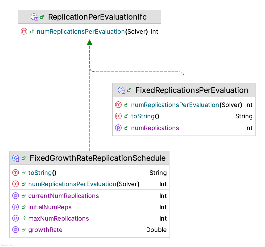
Figure 10.22: Replications Per Evaluation Hierarchy

GenerateNeighborIfc interface - This functional interface can be used by solvers to specify how to generate a neighbor relative to the supplied input. The ensureFeasibility parameter should indicate if the generation method should ensure that the returned input map is feasible with respect the constraints of the problem.

fun interface GenerateNeighborIfc {

    fun generateNeighbor(inputMap: InputMap, solver: Solver, ensureFeasibility: Boolean) : InputMap

}

NeighborSelectorIfc interface - This functional interface defines functions for selecting a neighbor (point) from a defined neighborhood represented as as set containing inputs. The supplied solver could be used to allow memory during the selection process.

fun interface NeighborSelectorIfc {

    fun select(neighborhood: Set<InputMap>, solver: Solver) : InputMap

}

SolutionQualityStoppingCriteriaIfc interface - This functional interface represents functions that define when to stop the iterative process based on the quality of the solution. As previously noted, the solutionQualityEvaluator property will be used when the stopping criteria is evaluated within the main loop. Examples of different ways to stop the algorithms will be presented during the discussion of specific algorithms. The solutionQualityEvaluator property provides the user with an approach to overriding the base behavior with different behavior rather than through sub-classing.

fun interface SolutionQualityEvaluatorIfc {

    fun isStoppingCriteriaReached(solver: Solver): Boolean

}

10.5.3 Miscellaneous Concepts in the `Solver` Class

This section presents some additional functionality within the Solver class that can be used when implementing specific algorithms. Figure 10.23 represents the properties associated with the Solver and StochasticSolver abstract base classes.

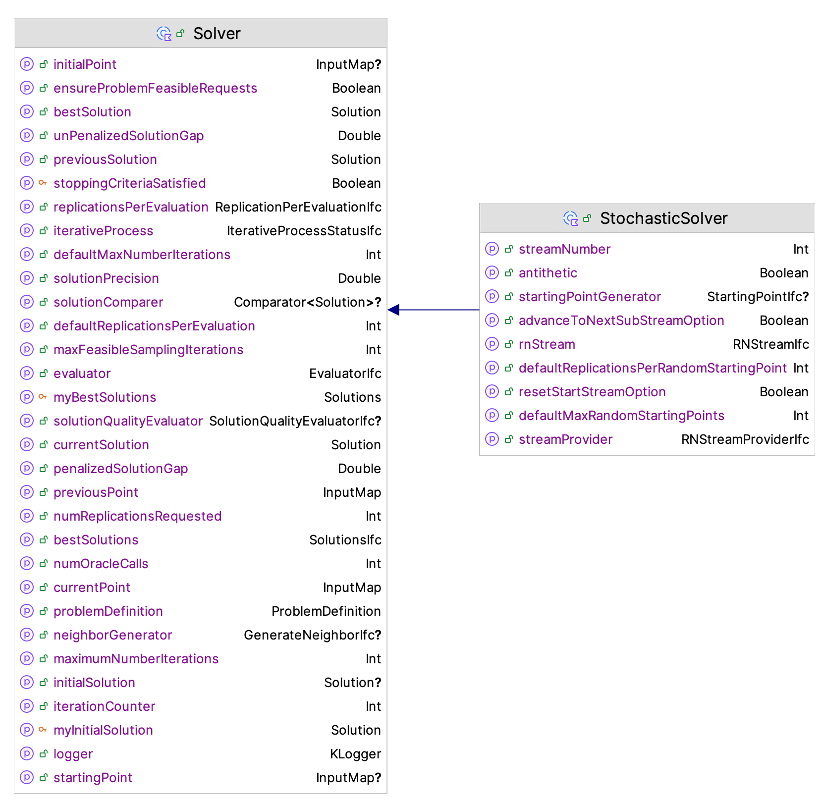
Figure 10.23: The Solution Class

The primary functionality to understand is how the Solver class keeps track of the solutions that it produces. The most important property to understand how to use is the currentSolution property. For this property, it is useful to see how the current solution is defined:

    var currentSolution: Solution = problemDefinition.badSolution()
        protected set(value) {
            // save the previous solution
            previousSolution = field
            // update the current solution
            field = value
            myBestSolutions.add(value)
        }

The current solution is initialized as a bad solution. Recall that a bad solution is a solution that is the worse possible solution for the problem. This can be retrieved via the ProblemDefinition class’s badSolution() function. The implementation of the solver algorithm should set the current solution during its search process. Notice that the previous solution is set during the assignment. This property provides access to the previous solution visited by the solver. Some solvers may compare the current solution with the previous solution as part of the stopping criteria evaluation process.

Also note that the myBestSolutions protected property is used to capture the newly assigned solution. The protected myBestSolutions property is an instance of the Solutions class. Figure 10.24 presents the SolutionsIfc interface and the Solutions class.

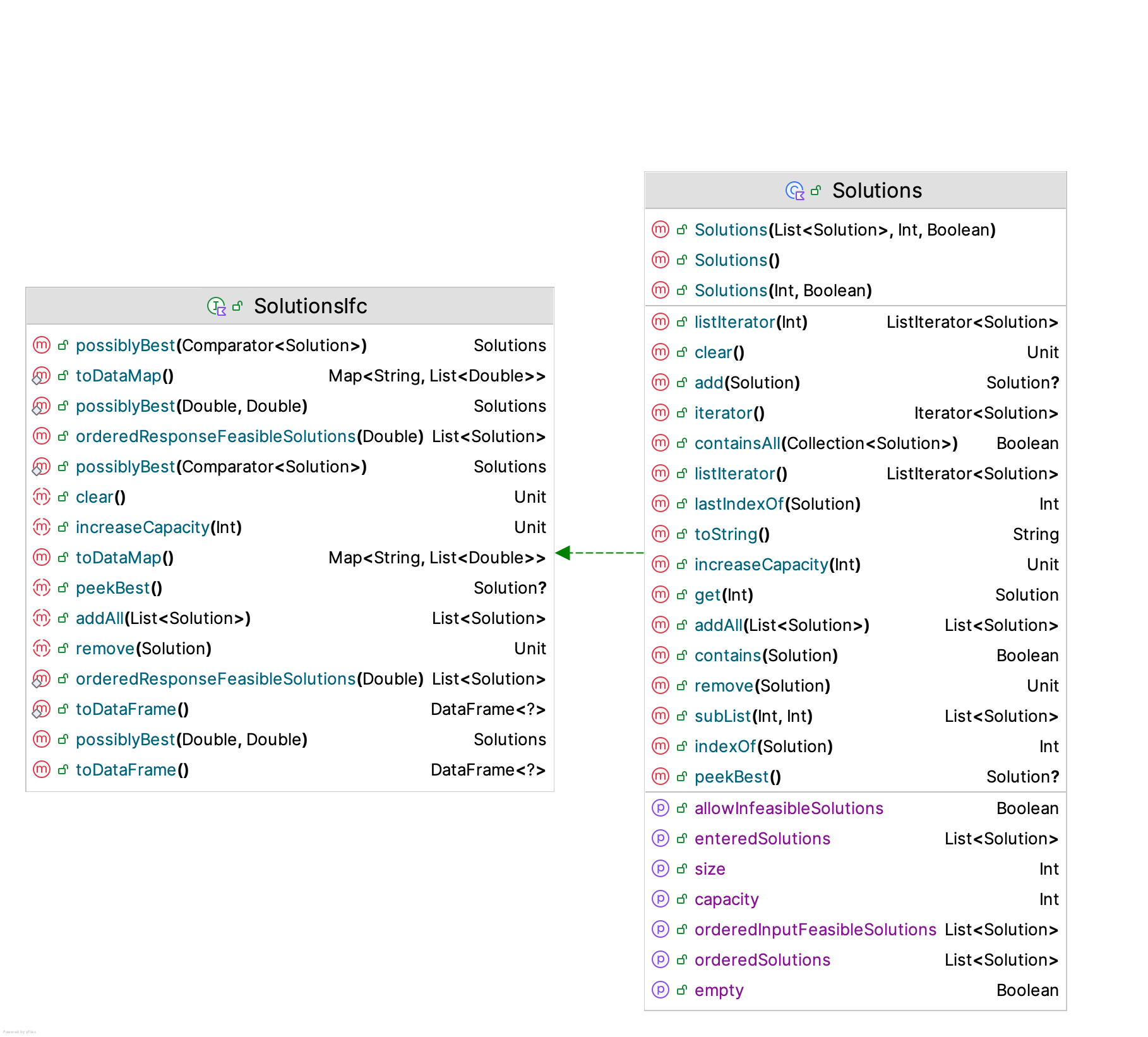
Figure 10.24: The Solutions Class

The SolutionsIfc implements the List<Solution> interface, which allows instances of the Solutions class to be treated as a list. The implementation of the Solutions class provides an ordering to the solutions based on the order in which they are added to the list and based on the value of the penalized objective function. The constructor of the Solutions class is presented in the following code.

class Solutions(
    capacity: Int = defaultCapacity,
    var allowInfeasibleSolutions: Boolean = false
) : SolutionsIfc

Conceptually, an instance of the Solutions class is like a cache, with a default capacity. It also controls whether it can store infeasible solutions. While the SolutionsIfc interface implements the List<Solution> interface, the implementation within the Solutions class allows mutability by providing specialized add(), addAll(), and remove() functions. Three functions facilitate extracting the best of the stored solutions.

peekBest(): Solution? - This function returns the solution with the lowest penalized objective function value.
possiblyBest(comparator: Comparator<Solution>): Solutions - This function returns a list of solutions that are possibly the best using the supplied comparator.
possiblyBest(level: Double = DEFAULT_CONFIDENCE_LEVEL,indifferenceZone: Double = 0.0): Solutions - This function returns solutions that could be considered best using a penalized objective function confidence interval comparator. The basic procedure is to select the smallest or largest solution as the best depending on the direction of the objective. Then, this procedure uses the best solution as the standard and compares all the solutions with it in a pair-wise manner. Any solutions that are considered not statistically different from the best solution are returned. The confidence interval is for each individual comparison with the best. Thus, to control the overall confidence, users will want to adjust the individual confidence interval level such that the overall confidence in the process is controlled as discussed in Section 5.7.2.

The property enteredSolutions returns the solutions in the order in which they occurred (i.e. the order in which they were added to the solutions). The properties orderedInputFeasibleSolutions and orderedSolutions return the solutions ordered by penalized objective function values.

In some situations, you may want to compare the effectiveness of different solvers for a problem. There are four properties of the Solver class that can help with this assessment process.

iterationCounter - The iterationCounter property counts the number of iterations performed by a solver. Since some solvers may used additional stopping criteria, this property can be used to assess the total number of iterations performed.
numOracleCalls - Each time a solver requests evaluations from the oracle, this property is incremented. It can be used to indicate how may simulation evaluations were performed. Since simulation evaluations can be computationally expensive, this property can help understand how efficient a solver is with respect to simulation evaluations.
numReplicationsRequested - Similar to the numOracleCalls property, this property totals the number of replications requested during the solver’s execution. This property can help understand how efficient a solver is in terms of its sampling.
iterativeProcess - This property references the underlying iterative process via the IterativeProcessStatusIfc interface. Figure 10.25 presents this interface. From the perspective of evaluating a solver’s efficiency, the beginExecutionTime and endExecutionTime properties can be used to compute the total time spent by the solver.

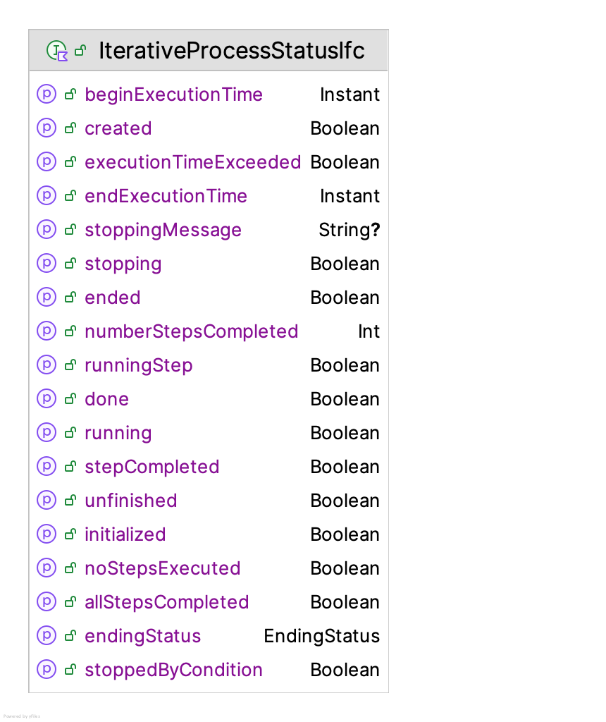
Figure 10.25: IterativeProcessStatusIfc Interface

The final concept to discuss involves classes that assist with checking for convergence. Recall that algorithms will select a candidate point and evaluate that point via the simulation oracle. For many algorithms, the selection of the point is driven by a process that may converge such that the same point (or nearly the same point) is repeatedly selected. We may choose to stop the algorithm if the same point is repeatedly selected. The SolutionChecker class is designed to hold and test if its contained solutions are all the same. Figure 10.26 presents the SolutionChecker class and the SolutionEqualityIfc interfaces.

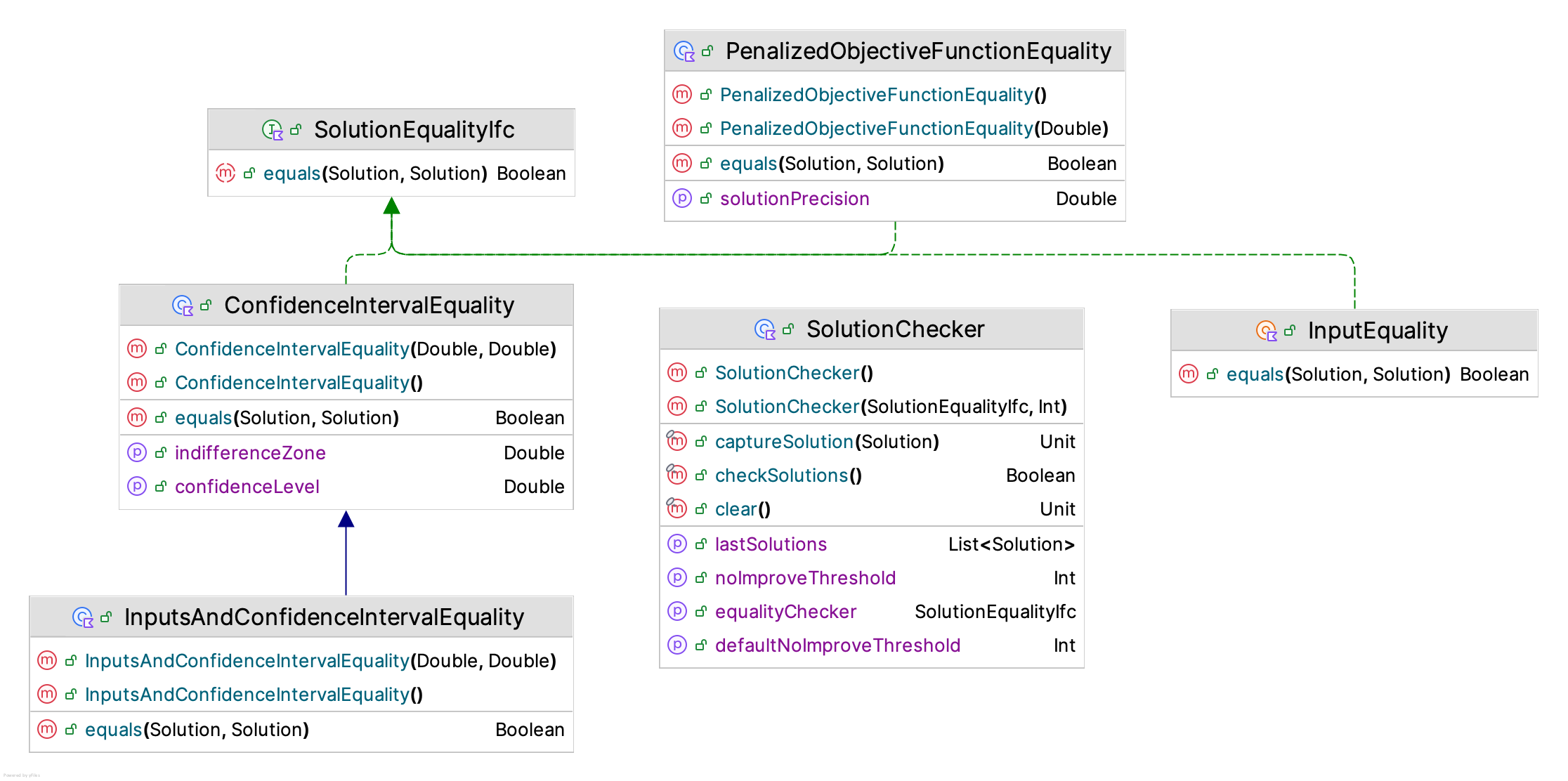
Figure 10.26: The Solution Checker Class

The purpose of the SolutionEqualityIfc interface is to provide a mechanism to check for the equality between two solutions. As can be noted in Figure 10.26 there are a variety of ways to define equality.

ConfidenceIntervalEquality - This class checks for equality between solutions based whether the confidence interval on the difference contains the indifference zone parameter. This is based on an approximate confidence interval on the difference between the unpenalized objective function values.
PenalizedObjectiveFunctionEquality - This class checks if the penalized objective function values are within some specified precision. The uncertainty of the values is not taken into consideration.
InputEquality This class indicates that two solutions are equal based only on the values of their inputs. If the solutions do not have the same inputs, then the penalized objective function is used to determine the ordering. Thus, two solutions are considered the same if they have the same input values, regardless of the value of the objective functions.
InputsAndConfidenceIntervalEquality - This class checks for equality between solutions based whether the confidence interval on the difference contains the indifference zone parameter and whether the input variable values are the same.

The SolutionChecker class uses an instance of the SolutionEqualityIfc interface to check if the elements that it holds all test as equal. The constructor requires a threshold value that represents the number of solutions to check. When the solution checker contains the specified number of solutions, the user can call the checkSolutions() function, which will return true if the all the contained solutions test as equal. The specified threshold limit also specifies the capacity. The checker will only hold the specified number of solutions.

class SolutionChecker(
    var equalityChecker: SolutionEqualityIfc = InputEquality,
    noImproveThreshold: Int = defaultNoImproveThreshold
)

An instance of the SolutionChecker class can be used as part of the logic for checking if the stopping criteria for the algorithm indicates if the algorithm should stop. Examples of this will be illustrated when covering specific algorithms.