10.6 Implemented Solvers
This section will overview the set of solvers provided within the KSL for use on simulation optimization problems. As shown in Figure 10.21, the following algorithms are available.
StochasticHillClimber- A stochastic hill climbing solver implements the idea of randomly moving through the search space. As new solutions are found, the current solution is updated if the next solution is better than the previous solution. Variations of stochastic hill climbing involve how to select points. It is one of the simplest algorithms to implement and it is still useful because in the limit, the algorithm will eventually visit the optimal solution.SimulatedAnnealing- Simulated annealing is a stochastic optimization algorithm that models the optimization process based on an analogy with a metallurgical annealing process. Popularized by (Kirkpatrick et al. 1983), simulated annealing has been widely used as a general purpose optimization methodology. For further background on simulation annealing, the interested reader should consider this on-line book.CrossEntropySolver- The cross-entropy method is a population based algorithm that is based on minimizing the cross-entropy between a target distribution and a parametric distribution. (De Boer et al. 2005) present a detailed tutorial on the cross-entropy method. The cross-entropy method is a general purpose meta-heuristic. While designed for deterministic optimization problems, the cross-entropy method has also been applied to stochastic optimization problems.RSplineSolver- The R-SPLINE method is presented in (Wang et al. 2013). This method is designed for integer-ordered (discrete) optimization problems. The overall theory guarantees convergence to locally optimal solutions.RandomRestartSolver- Many solvers require an initial starting point. The algorithm’s final solution may be sensitive to the choice of the initial starting point. A common strategy is to repeat the algorithm at different starting points and selecting the solution that is best across the starting points. This solver permits other solvers to be called repeatedly for randomly selected starting points.
The previously discussed framework should allow users to implement their own solvers. This section discusses some of the key features of the provided solvers, which may be of interest when using the solvers. Since the StochasticHillClimber solver was already discussed, it will not be discussed here. We will start with the classic simulated annealing algorithm.
10.6.1 Simulated Annealing
Simulated annealing is an optimization approach that is based on the concepts of Markov Chain Monte Carlo (MCMC) (see Section 9.3.4). As presented in Chapter 9, MCMC can be used to generate from arbitrarily specified multivariate distributions. Simulated annealing exploits the MCMC sampling process to find a mode of density function, \(f(x)\). This mode represents a point where \(f(x)\) is maximized. The process produces a sequence of density functions \(f_T(x) \propto [f(x)]^{1/T}\), where \(T\) denotes the temperature of the distribution. The sampling process produces a Markov chain such that the generated values \(x_k\) are from the distributions \(f_{T_k}\) for decreasing temperatures \(T_1, T_2, \dots\). As the temperatures decrease, the distributions converge to a highly peaked distribution, where the peak is at the maximum of the distribution, \(f\). The point causing the peak will also be the solution to the optimization problem. A key factor in this process is the cooling schedule that determines the temperature sequence.
As we can see from the constructor, the user must supply the problem definition, the evaluator and values for the key parameters of the annealing process:
initialTemperature- The starting temperature for the process.coolingSchedule- An implementation of theCoolingScheduleIfcinterface to determining the temperature at each iteration.stoppingTemperature- If the current temperature goes below this value, the algorithm will stop.
class SimulatedAnnealing @JvmOverloads constructor(
    problemDefinition: ProblemDefinition,
    evaluator: EvaluatorIfc,
    initialTemperature: Double = defaultInitialTemperature,
    var coolingSchedule: CoolingScheduleIfc = ExponentialCoolingSchedule(initialTemperature),
    stoppingTemperature: Double = defaultStoppingTemperature,
    maxIterations: Int = defaultMaxNumberIterations,
    replicationsPerEvaluation: ReplicationPerEvaluationIfc,
    streamNum: Int = 0,
    streamProvider: RNStreamProviderIfc = KSLRandom.DefaultRNStreamProvider,
    name: String? = null
) : StochasticSolver(problemDefinition, evaluator, maxIterations, replicationsPerEvaluation, streamNum, streamProvider, name) {
Pseudo-code for the overall algorithm is as follows:
1. Initialize the solution and the temperature
2. While not converged
  2.1. Generate a possible solution based on some probabilistic process
  2.2. Calculate the change in the objective function
  2.3. If an improvement or acceptance probability is met
    2.3.1 accept the new solution
  2.4 Reduce the temparture according the cooling schedule
3. Return the best solution found
A unique aspect of the simulated annealing process is that a solution that is not an improvement over the current solution can be accepted as the current solution. This permits exploration of the solution space. As the temperature decreases it becomes less likely that non-improving solutions will be accepted.
Although the algorithm will stop when the maximum number of iterations is met, implementations often use approaches that stop when consecutive objective function values are less than some tolerance, when the temperature becomes too small, or when the objective function value has not changed after a number of iterations.
The SimulatedAnnealing class implements the initializeIterations(), mainIteration(), and the isStoppingCriteriaSatisfied() functions. The mainIteration() function follows closely the outlined pseudo-code:
    override fun mainIteration() {
        // generate a random neighbor of the current solution
        val nextPoint = nextPoint()
        // evaluate the point to get the next solution
        val nextSolution = requestEvaluation(nextPoint)
        // calculate the cost difference
        costDifference = nextSolution.penalizedObjFncValue - currentSolution.penalizedObjFncValue
        // if the cost difference is negative, it is automatically an acceptance
        if (costDifference < 0.0) {
            // no need to generate a random variate
            currentSolution = nextSolution
            lastAcceptanceProbability = 1.0
            logger.trace { "Solver: $name : solution improved to $nextSolution" }
        } else {
            // decide whether an increased cost should be accepted
            val u = rnStream.randU01()
            lastAcceptanceProbability = acceptanceProbability(costDifference, currentTemperature)
            if (u < lastAcceptanceProbability) {
                currentSolution = nextSolution
                logger.trace { "Solver: $name : non-improving solution was accepted: $nextSolution" }
            } else {
                // stay at the current solution
                logger.trace { "Solver: $name : rejected solution $nextSolution" }
            }
        }
        // update the current temperature based on the cooling schedule
        currentTemperature = coolingSchedule.nextTemperature(iterationCounter)
        // capture the last solution
        solutionChecker.captureSolution(currentSolution)
    }
The implementation uses the nextPoint() function from the StochasticSolver class to generate a neighbor of the current point. The new point is evaluated via the simulation oracle. Then, the objective function cost difference is computed. If there is an improvement, the next solution is automatically accepted as the current solution. If the proposed point caused an increase in the objective function, then the algorithm randomly generates a U(0,1) variate and compares it to the current acceptance probability. If the randomly generated value is less than the acceptance probability, the proposed point is accepted; otherwise, the current solution stays the same. The acceptance probability criteria is based on the Boltzman distribution and is a function of the objective function difference and the current value of the temperature.
    fun acceptanceProbability(costDifference: Double, temperature: Double) : Double {
        require(temperature > 0.0) { "The temperature must be positive" }
        return if (costDifference <= 0.0) {
            1.0
        } else {
            exp(-costDifference / temperature)
        }
    }
The current temperature is computed based on a user definable function to implement the cooling schedule. The default implementation uses an exponential cooling schedule. The ksl.solvers.algorithms package also provides implementations for linear and logarithmic cooling schedules.
class ExponentialCoolingSchedule(
    initialTemperature: Double,
    val coolingRate: Double = defaultCoolingRate
) : CoolingSchedule (initialTemperature)  {
    init {
        require(coolingRate > 0.0) { "Cooling rate must be positive" }
        require(coolingRate < 1.0) { "Cooling rate must be less than 1.0" }
    }

    override fun nextTemperature(iteration: Int): Double {
        require(iteration > 0) { "The iteration must be positive. It was $iteration." }
        return initialTemperature * coolingRate.pow(iteration)
    }
}
The implementation of the SimulatedAnnealing class uses an instance of the previously discussed SolutionChecker class as part of the stopping criteria to check if the last 5 solutions are the same or if the temperature has become too small.
10.6.2 Cross Entropy
Similar in some respect to simulated annealing, the cross-entropy method is a stochastic optimization procedure that can be applied to both deterministic and stochastic optimization problems. The basic procedure is described in (De Boer et al. 2005) and can be characterized as a population based approach because it uses a sample of the search space to define an elite population. Cross-entropy uses rare-event simulation techniques to cause the parameters of a sampling distribution to converge to the desired solution of the related optimization problem. The cross-entropy method can be applied to optimization problems involving both continuous and discrete variables.
As presented in (Rubinstein and Kroese. 2017) the basic cross-entropy algorithm is as follows. The value \(\rho\) is called the elite percentage. The algorithm presented here is in terms of minimizing the objective function.
- Let \(k=0\) be the iteration counter. Initialize \(\hat{v}_0\) as the initial parameters of some density function \(f(\cdot;v_{k})\). Let \(N^e = \lceil \rho N \rceil\) be the size of the elite sample. Let \(N\) be the size of the cross-entropy population.
- Repeat
- Generate a sample \(\vec{X}_1, \vec{X}_2, \dots, \vec{X}_N\) from \(f(\cdot;v_{k-1})\).
- Calculate the performance \(G(\vec{X}_1), G(\vec{X}_2),\dots, G(\vec{X}_N)\).
- Order the performance from smallest to largest: \(G_{(1)}, G_{(2)},\dots, G_{(N)}\)
- Let \(\hat{\gamma}_k = G_{(N^e)}\)
- Use the same sample \(\vec{X}_1, \vec{X}_2, \dots, \vec{X}_N\) and solve a corresponding stochastic program, see (Rubinstein and Kroese. 2017) resulting in the estimated parameters of the sampling distribution \(\tilde{v}_k\).
- Update the parameters according to: \(\hat{v}_k = \alpha \tilde{v}_k + (1-\alpha) \hat{v}_{k-1}\).
- k = k + 1
- Until : a stopping criteria is met.
The stochastic program mentioned in step 2.5 of the algorithm is essentially the estimation of the parameters of \(f(\cdot;v_{k})\) via the maximum likelihood method based on the elite sample at each iteration. The elite sample consists of those \(\vec{X}_i\) such that \(G(\vec{X}_i) \ge \hat{\gamma}_k\). (Rubinstein and Kroese. 2017) recommend that the procedure be stopped if for some \(k \ge d\), say \(d=5\), when \(\hat{v}_k = \hat{v}_{k-1} = \cdots = \hat{v}_{k-d}\).
The choice of the density function \(f(\cdot;v_{k})\) is an important aspect of the algorithm because the parameters converge to the optimal solution of the associated optimization problem. Actually, similar to simulated annealing, the sequence of density functions \(f(\cdot;\hat{v}_{1}),f(\cdot;\hat{v}_{2}), \dots\) converges to a degenerate distribution assigning all probability to a single point \(x_k\), for which the objective function value is greater than or equal to \(\hat{\gamma}_k\). This point represents the solution to optimization problem. (De Boer et al. 2005) discuss different possibilities for the density function. The normal distribution is recommended for continuous optimization problems while the Bernoulli distribution has been used for discrete optimization problems. The critical aspect of this choice is the ability to easily compute the maximum likelihood estimates for the parameters of the distribution based on the elite sample.
The KSL implementation of the cross-entropy solver follows this general algorithm and builds from the StochasticSolver class. You must specify an instance of the CESamplerIfc interface or accept the default of a sampler based on the multivariate normal distribution. The stopping criteria is based on providing an instance of the InputsAndConfidenceIntervalEquality class, which implements the SolutionEqualityIfc interface. This will test if \(\hat{v}_k = \hat{v}_{k-1} = \cdots = \hat{v}_{k-d}\) is true based on equal values of inputs and a comparison of the solutions based on confidence interval comparisons with the best solution.
class CrossEntropySolver @JvmOverloads constructor(
    problemDefinition: ProblemDefinition,
    evaluator: EvaluatorIfc,
    val ceSampler: CESamplerIfc = CENormalSampler(problemDefinition),
    maxIterations: Int = ceDefaultMaxIterations,
    replicationsPerEvaluation: ReplicationPerEvaluationIfc,
    solutionEqualityChecker: SolutionEqualityIfc = InputsAndConfidenceIntervalEquality(),
    name: String? = null
) : StochasticSolver(problemDefinition,
    evaluator, maxIterations,
    replicationsPerEvaluation, ceSampler.streamNumber,
    ceSampler.streamProvider, name
)
The implementation uses the instance of the CESamplerIfc interface to generate the points \(\vec{X}_1, \vec{X}_2, \dots, \vec{X}_N\) via the function call ceSampler.sample(sampleSize()) within the mainIteration() function. The function sampleSize() computes the size, \(N\), of the cross-entropy population at each iteration. Then, the solver requests the evaluation of those points to produce the estimated performance of the objective function, \(G(\vec{X}_1), G(\vec{X}_2),\dots, G(\vec{X}_N)\).
    override fun mainIteration() {
        // Generate the cross-entropy sample population
        val points = ceSampler.sample(sampleSize())
        // Convert the points to be able to evaluate.
        val inputs = problemDefinition.convertPointsToInputs(points)
        // request evaluations for solutions
        val evaluations = requestEvaluations(inputs)
        val results = evaluations.values.toList()
        if (results.isEmpty()) {
            // Returning will cause no updating on this iteration.
            // New points will be generated for another try on the next iteration.
            return
        }
        // At least one result, so proceed with processing.
        // Process the results to find the elites. This should fill myEliteSolutions.
        myEliteSolutions = findEliteSolutions(results)
        // convert elite solutions to points
        val elitePoints = extractSolutionInputPoints(myEliteSolutions)
        // update the sampler's parameters
        ceSampler.updateParameters(elitePoints)
        // specify the current solution
        currentSolution = myEliteSolutions.first()
        // capture the last solution
        solutionChecker.captureSolution(currentSolution)
    }
The elite solutions are found via the call to findEliteSolutions() and the points associated with the elite solutions are used to update the parameters of the cross-entropy sampler. The best solution from the elite sample is used to represent the current solution. Just like the simulated annealing algorithm, the cross-entropy implementation uses an instance of the SolutionChecker class to remember the last \(d\) solutions and to stop when they have converged.
There are a number of key issues that must be implemented for the cross-entropy method.
- How large should the population (\(N\)) be?
- What should the elite percentage \(\rho\) be? Alternatively, what should be the size of the elite sample?
- What parametric family of distributions should be used for the sampling distribution?
- How to initialize the parameters of the sampling distribution?
- How to update the parameters of the sampling distribution?
- What should the value of the smoothing parameter \(\alpha\) be?
(De Boer et al. 2005) recommends that the size of the population, \(N\), be related to the dimension of the problem. If we let \(K\) be the number of parameters that need to be estimated for the sampling distribution, then (De Boer et al. 2005) recommends \(N=cK\), where \(c\) is a number between 1 and 10. For example, if the sampling distribution family is the normal distribution, we must estimate two parameters for each input variable, that is \((\mu_i, \sigma_i)\) for \(i=1,2,\dots, |I|\). Thus, \(K=2*|I|\). The KSL provides more flexibility with respect to determining the population size. As previously mentioned, the implementation provides the sampleSize() function, which can be customized by providing an implementation of the SampleSizeFnIfc functional interface.
The base implementation will use a supplied sample size function or use the value of the ceSampleSize property.
The value of the ceSampleSize property is based on a user changeable default value or a recommended sample size based on the size of a sample needed to adequately estimate the quantile of a distribution.
    var ceSampleSize: Int = minOf(recommendCESampleSize(), defaultMaxCESampleSize)
        set(value) {
            require(value >= defaultMinCESampleSize) { "The CE sample size must be >= $defaultMinCESampleSize" }
            field = minOf(value, defaultMaxCESampleSize)
        }
The recommended cross-entropy sample size is based on the results presented in (Chen and Kelton 1999) and is implemented in the recommedCESampleSize() companion function.
        fun recommendCESampleSize(
            elitePct: Double = defaultElitePct,
            ceQuantileConfidenceLevel: Double = defaultCEQuantileConfidenceLevel,
            maxProportionHalfWidth: Double = defaultMaxProportionHalfWidth,
        ): Int
The computed sample size may be sufficient to adequately estimate the quantile associated with the desired elite percentage using a desired quantile confidence level and an adjusted half-width bound for the associated quantile proportion. Defaults are provided for each of these parameters.
Lastly, the KSL cross-entropy implementation permits customization of the size of the elite sample. In some situations, you may want to vary the size of the elite sample as the algorithm progresses to improve estimation of the parameters of the sampling distribution. The KSL implementation provides the eliteSize() function for this purpose.
    fun eliteSize(): Int {
        return eliteSizeFn?.eliteSize(this) ?: maxOf(ceil(elitePct * ceSampleSize).toInt(),
            defaultMinEliteSize)
    }
Note that a user can supply an instance of the EliteSizeIfc functional interface, which simply promises to compute the size of the elite sample.
The implementation of the eliteSize() function will use a supplied function specified by the eliteSizeFn property or determine the size based on the specified elite percentage.
The questions associated with the sampling distribution and the updating of its parameters should be addressed by the choice of the implementation of the CESamplerIfc interface chosen for the algorithm.
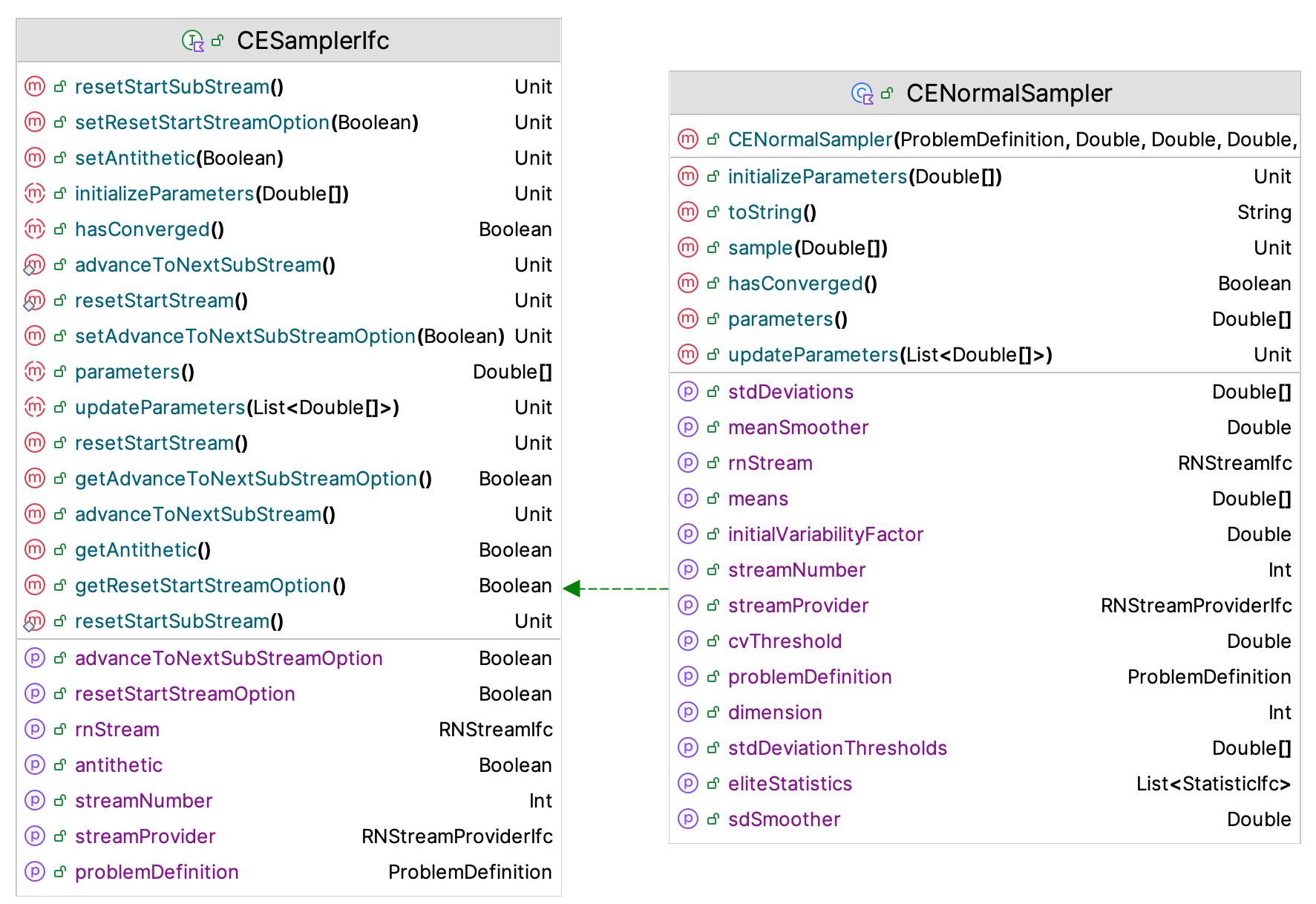
Figure 10.27: CESamplerIfc Interface
Figure 10.27 presents the CESamplerIfc interface and the CENormalSampler class, which implements the sampling process based on the normal distribution. Note that the CESamplerIfc interface implements the MVSampleIfc and RNStreamControlIfc interfaces. Thus, it can act as a multivariate sampler and can control the underlying random number stream. The four most relevant functions are:
updateParameters(elites: List<DoubleArray>)- This function should update the parameters based on the points from the elite sample (held in a list of double arrays).parameters(): DoubleArray- This function returns the current parameter values.initializeParameters(values: DoubleArray)- This function is used to specify the initial values of the parameters.hasConverged(): Boolean- This function should return true if the parameters of the underlying sampling distribution are considered converged.
The initialization of the parameters of the cross-entropy sampling distribution is interesting because we do not have any knowledge from an elite sample when the algorithm starts. In essence, this is like determining the starting point of the optimization problem. For the CENormalSampler class, the implementation uses a randomly generated point in the solution space as the specification of the means of the multivariate normal distribution. Then, the input range of each point is used to approximate the initial values of the standard deviations for the distributions. The standard approximation for the standard deviation as a function of the range (\(R\)) is used: \(\sigma = R/4\). Thus, input variables that have a wider range of possible values start off with a higher variance parameter. The means associated with the normal distribution will converge to the recommended solution, while the standard deviations will continue to get closer and closer to zero as the process converges to a degenerate distribution.
As noted in Figure 10.27, the CENormalSampler class requires the specification of the smoothing constant, \(\alpha\), for both the mean and the standard deviation parameters. The user also has the ability to specify more or less variability via the initialVariabilityFactor property, which will be used to multiply the approximated initial values for the standard deviation parameters. Its default value is 1.0. The user must also specify the cvThreshold parameter value. This threshold is used to test if the parameters have converged. The default implementation computes the coefficient of variation of the parameters and if the coefficient of variation goes below this threshold, then the parameter is consider to have converged. If all the parameters have converged, then the hasConverged() function will return true. The default coefficient of variation threshold is set to \(0.03\).
Updating the parameters of the normal sampler is easy. We can just use the sample average and sample standard deviation of the elite points associated with the elite sample as the new estimates, and then smooth those estimate using the smoothing constants. Based on the recommendations from (De Boer et al. 2005), the default smoothing constants are set to \(0.85\). The KSL only supplies the CENormalSampler because testing has indicated that it performs okay for both discrete and continuous problems. Users can implement the defined interfaces if they require other parametric distributions.
10.6.3 R-SPLINE
This section will present an overview of the R-SPLINE algorithm discussed in (Wang et al. 2013). Since that paper has substantial details of the algorithm, the emphasis in this presentation will be on how the ksl.simopt package facilitates its implementation. As previously noted, the R-SPLINE algorithm is for discrete integer ordered optimization problems. If the user attempts to solve a problem that is not integer ordered, the R-SPLINE implementation will report an illegal argument exception for the problem definition parameter.
As a StochasticSolver, the RSplineSolver class requires a specification of the replications per evaluation and an implementation of a stopping criteria. Similar to the cross-entropy method, the R-SPLINE implementation also uses the InputsAndConfidenceIntervalEquality class for checking it the algorithm should stop. This is different than the approaches recommended in (Wang et al. 2013). Unique to the R-SPLINE algorithm is that the algorithm does not use a fixed replication sampling mechanism but rather the number of replications per evaluation will grow as the number of iterations increases. This is an important aspect of the theory behind the algorithm to justify claims that in the limit the algorithm will converge to local neighborhood optimal solutions.
class RSplineSolver @JvmOverloads constructor(
    problemDefinition: ProblemDefinition,
    evaluator: EvaluatorIfc,
    maxIterations: Int = defaultMaxNumberIterations,
    replicationsPerEvaluation: FixedGrowthRateReplicationSchedule,
    solutionEqualityChecker: SolutionEqualityIfc = InputsAndConfidenceIntervalEquality(),
    streamNum: Int = 0,
    streamProvider: RNStreamProviderIfc = KSLRandom.DefaultRNStreamProvider,
    name: String? = null
) : StochasticSolver(problemDefinition, evaluator, maxIterations,
    replicationsPerEvaluation, streamNum, streamProvider, name)
The R-SPLINE algorithm combines three ideas: 1) piece-wise linear interpolation search, 2) discrete neighborhood enumeration, and 3) retrospective solving of a sequence of sample path problems with an increasing sample size using the previous solution as the starting point for the next problem. (Wang et al. 2013) specifies algorithm 1 of R-SPLINE as
- Set \(X^{*}_{0} = x_0\)
- for \(k=1,2,\dots\)
- \(X^{*}_{k} = SPLINE(X^{*}_{k-1}, m_k, b_k)\)
- end for
The sequences \(m_k\) and \(b_k\), specify the sample size for the \(k^{th}\) iteration and \(b_k\) is the limit on the number of simulation evaluation calls. As you can see the mainIteration() function represents this algorithm. (Wang et al. 2013) recommends \(m_{k+1} = \lceil 1.1m_k \rceil\), which increases the sample size by 10 percent for each iteration.
    override fun mainIteration() {
        // The initial (current) solution is randomly selected or specified by the user.
        // It will be the current solution until beaten by the SPLINE search process.
        // Call SPLINE for the next solution using the current sample size (m_k) and
        // current SPLINE oracle call limit (b_k).
        val splineSolution = spline(
            currentSolution,
            rSPLINESampleSize, splineCallLimit
        )
        currentSolution = splineSolution
        // capture the last solution
        solutionChecker.captureSolution(currentSolution)
    }
The SPLINE function is fairly complex. Given a specification of the sample size for the iteration, \(m_k\), the supplied solution may need additional replications evaluated, which will result in a new estimated solution. Then, an inner loop of the spline searching process commences. This involves two phases. First, a search of a piece-wise linear interpolation of the objective function and then a search of the neighborhood resulting from the piece-wise linear interpolation search. The details of this process can be found as algorithm 2 in (Wang et al. 2013).
    private fun spline(
        initSolution: Solution,
        sampleSize: Int,
        splineCallLimit: Int
    ): Solution {
        require(initSolution.isInputFeasible()) { "The initial solution to the SPLINE function must be input feasible!" }
        // use the initial solution as the new (starting) solution for the line search (SPLI)
        var newSolution = if (sampleSize > initSolution.count){
            requestEvaluation(initSolution.inputMap, sampleSize)
        } else {
            initSolution
        }
        // save the starting solution
        val startingSolution = newSolution
        // initialize the number of oracle calls
        var splineOracleCalls = 0
        for(i in 1..splineCallLimit){
            // perform the line search to get a solution based on the new solution
            val spliResults = searchPiecewiseLinearInterpolation(newSolution, sampleSize)
            // SPLI cannot cause harm
            val neStartingSolution = if (compare(spliResults.solution, newSolution) <= 0){
                spliResults.solution
            } else {
                newSolution
            }
            // search the neighborhood starting from the SPLI solution
            val neSearchResults = neighborhoodSearch(neStartingSolution, sampleSize)
            splineOracleCalls = splineOracleCalls + spliResults.numOracleCalls + neSearchResults.numOracleCalls
            newSolution = neSearchResults.solution
            // if the candidate solution and the NE search starting solution are the same, we can stop
            if ((neStartingSolution == neSearchResults.solution) || compare(neStartingSolution, neSearchResults.solution) == 0) {
                break
            }
        }
        // Check if the starting solution is better than the solution from the SPLINE search.
        return if (compare(startingSolution, newSolution) < 0) {
            startingSolution
        } else {
            // The new solution might be better, but it might be input-infeasible.
            if (newSolution.isInputFeasible()) {
                newSolution
            } else {
                // not feasible, go back to the last feasible solution
                startingSolution
            }
        }
    }
The piece-wise linear search process proceeds roughly as follows. Given a point, \(x\in\mathbb{R}^d \setminus \mathbb{Z}^d\) in the space, consider the \(2^d\) integer points that are the vertices of the hyper-cube that contains \(x\). The algorithm chooses \(d+1\) vertices so that the convex hull of the points form a simplex that contains \(x\). An interpolation of the objective function evaluated at the points of the simplex provides a linear interpolation function from which an estimate of the gradient associated with the objective function can be computed. The gradient is used to determine a direction and then a linear line search is used to proceed in the specified direction.
This process continues until no improvement can be made in the direction of search at which point the piece-wise linear search process returns with the last point associated with its search. Then, an Von Neumann neighborhood is found around the the returned point and the neighborhood is enumerated and the best solution from the enumeration process returned. If the enumeration solution is the same as the solution from the piece-wise linear search process then the SPLINE process stops; otherwise, another SPLINE cycle occurs. The cycles will stop when the number of spline calls is reached or the SPLINE search and the enumeration search are the same. An important aspect of the gradient estimation process is that common random numbers are used when evaluating the points that form the simplex around the proposed point. To implement these procedures the KSL provides the following functions.
searchPiecewiseLinearInterpolation(solution: Solution, sampleSize: Int): SPLIResults- This is essentially algorithm 4 of (Wang et al. 2013).piecewiseLinearInterpolation(solution: Solution,sampleSize: Int,perturbation: Double): PLIResults- This is algorithm 3 of (Wang et al. 2013).perturb(point: DoubleArray, perturbation: Double): DoubleArray- This is the PERTURB function mentioned in (Wang et al. 2013).neighborhoodSearch(solution: Solution,sampleSize: Int): NESearchResults- This function implements the enumeration and search of the neighborhood defined in the SPLINE process.
10.6.4 Randomized Restart Solvers
In general, optimization algorithms rely on a starting point to initialize the search process. The performance of the algorithm may be sensitive to the choice of the starting point, which may cause the search process to converge to a local optimal or to limit the exploration of the search space. A random restart solver is a solver that starts another solver using different randomly generated starting points. As we can see from the constructor of the RandomRestartSolver class, the user must supply a solver.
class RandomRestartSolver(
    val restartingSolver: Solver,
    maxNumRestarts: Int = defaultMaxRestarts,
    streamNum: Int = 0,
    streamProvider: RNStreamProviderIfc = KSLRandom.DefaultRNStreamProvider,
    name: String? = null
) : StochasticSolver(
    restartingSolver.problemDefinition, restartingSolver.evaluator, maxNumRestarts,
    restartingSolver.replicationsPerEvaluation, streamNum, streamProvider, name
)
The mainIterations() function is very straightforward. Since we want independent solutions, we clear a solution cache if it is being used. Then, a new starting point is generated and assigned as the starting point for the solver. The solver is executed for all of its iterations (or until its stopping criteria are met). The best solution from the execution of the solver is captured.
    override fun mainIteration() {
        // clear the evaluator cache between randomized runs, but allow caching during the run itself
        // this will cause new replications to be generated
        if (clearCacheBetweenRuns){
            evaluator.cache?.clear()
        }
        // randomly assign a new starting point
        val startPoint = startingPoint()
        restartingSolver.startingPoint = startPoint
        // run the solver until it finds a solution
        restartingSolver.runAllIterations()
        numOracleCalls = numOracleCalls + restartingSolver.numOracleCalls
        numReplicationsRequested = numReplicationsRequested + restartingSolver.numReplicationsRequested
        // get the best solution from the solver run
        val bestSolution = restartingSolver.bestSolution
        currentSolution = bestSolution
    }
Thus, repeated executions of the solver start with a different starting point and may produced different solutions. In the next section, we will illustrate how to set up solvers to solve an optimization problem.