10.2 Simulation Optimization Methods
The field of simulation optimization encompasses the use of computer simulation models as part of an optimization search process. As was discussed in Chapter 1, simulation models take on numerous forms including deterministic/stochastic, static/dynamic, and continuous/discrete models. Each of these forms may require specialized optimization methods in order to utilize the simulation model as part of the search process. Consider Figure 10.8 within the context of optimization, we can visualize how a simulation model (the box labeled “Model for Predicting System Performance” in the figure), can be used as part of an optimization process.
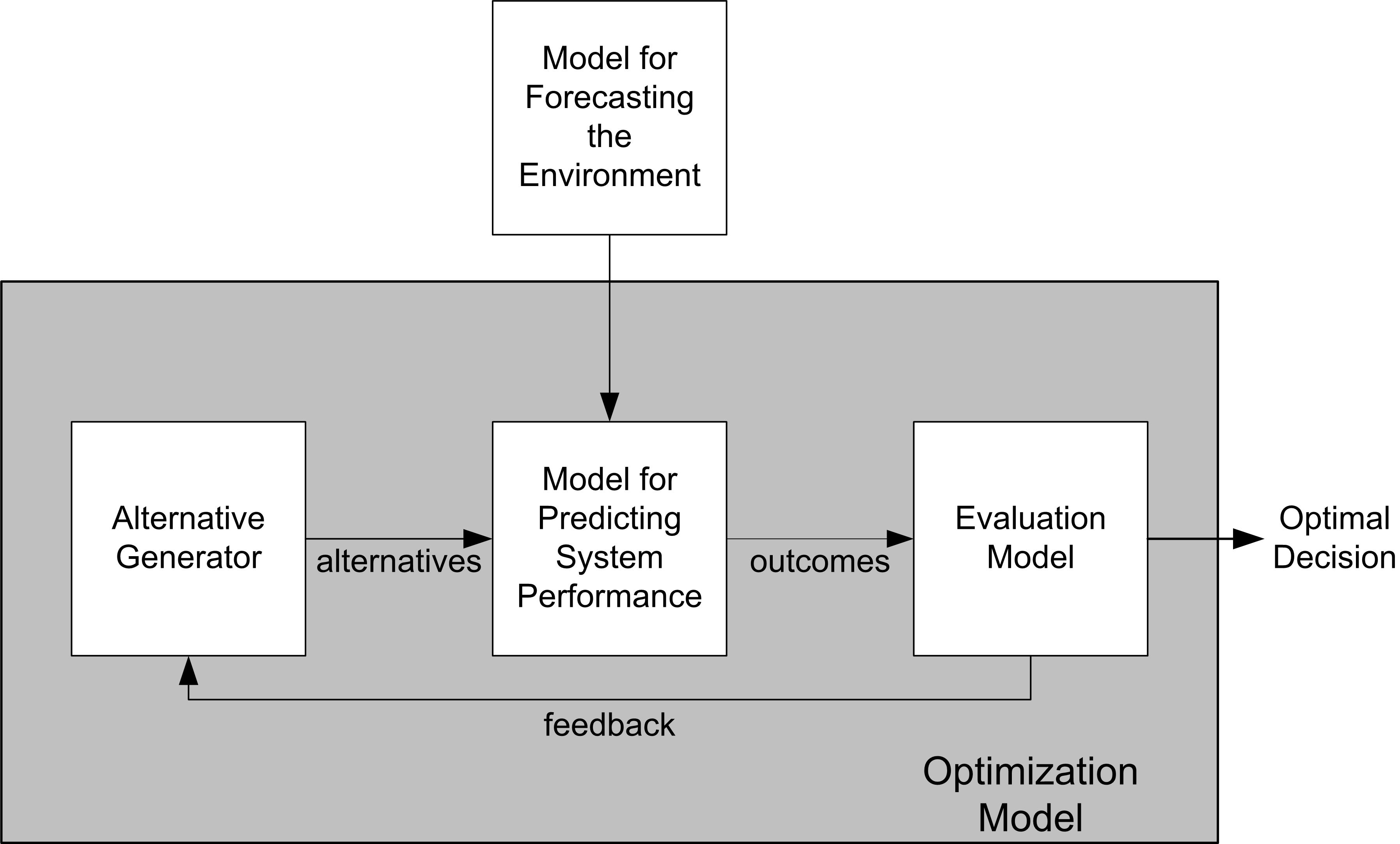
Figure 10.8: Simulation as Part of an Optimization Process
The dark-shaded area of Figure 10.8 represents an optimization model. In general form, an optimization model has the ability to generate candidate alternatives which are evaluated by the simulation model. The output from the simulation model is used by some kind of “evaluation model”, typically an objective function, but the evaluation may in fact constitute multiple objectives. The optimization model is an iterative process that continues generating alternatives for evaluation and evaluating the alternatives until the desire solution quality is achieved. In Chapter 5 and in Section 10.1 of this chapter, the decision maker or analyst is the “optimization model”. That is, it is up to the analyst to determine the set of alternatives to evaluate and to make conclusions about which are to be recommended. This section will describe processes for which the optimization model presented in Figure 10.8 is automated in some fashion via algorithms.
From this context, we can conclude that simulation optimization has substantial areas that can be extremely complex, theoretical, yet with many practical applications. Thus, for the purposes of this chapter, we will not attempt to present a discussion of the wide-range of algorithms and topics that underpin the area of simulation optimization. Excellent tutorials already exist on this extensive topic. We refer the interested reader to (Jian and Henderson 2015), (Pasupathy and Ghosh 2013), (Nelson 2014), and (Spall 2012) for introductions. In addition, the focus of this section is to present the practical concepts that users of such algorithms need for understanding some of the trade-offs and issues that occur when using the algorithms.
While some algorithms offer theoretical proofs of convergence, that issue is by-passed within this presentation. The focus here is how to use the algorithm to obtain useful solutions within a reasonable time-frame. In this regard, the concepts presented in (Henderson 2021) are relevant because we are interested in algorithms that are well equipped to tackle problems with little structure and which provide solutions that improve an objective function over practical time-scales. In general, we desire algorithms that are general, relatively easy to use or setup, and can be applied in a variety of contexts.
With respect to this chapter, the general form of a simulation optimization problem can be written as:
\[ \min_{x\in S} g(x) \] where \(g\) is an objective function, \(x\) represents the decision variables, with constraints \(x \in S\). The objective function can be linear or non-linear and the decision variables may be continuous or discrete. The objective function and/or constraints may involve randomness and one (or both) require a simulation model for evaluation. That is, the simulation model is like a “black-box” to which we can provide inputs and then observe outputs for use in the optimization process.
Because our use case primarily involves systems that include randomness, a common method is to present the formulation in terms of expected values, where the objective function \(g\) and the constraint set \(S\) is written as:
\[ g(x) = E[g(x, \xi_i)] \\ S = \{x: E[h(x, \xi_i)] \leq 0 \} \] where \(\xi_i\) represents the randomness associated with the \(i^{th}\) observation (sample) for the objective function, \(g(\cdot)\) and \(h(\cdot)\) represents a performance measure, both, estimated from the simulation. In addition, we must note that while the formulation does not indicate this explicitly, the inputs, \(x\), are vector-valued and the responses \(h(\cdot)\) may also be vectors. A wide variety of formulations are also seen in the literature. See (Jian and Henderson 2015) and (Pasupathy and Ghosh 2013) for further characterizations. The point here is that the general formulation is quite challenging and even more so because uncertainty (randomness) is involved.
The KSL provides a framework of classes that permit the construction of problem instances, which can be solved via different optimization algorithms as illustrated in Figure 10.8. The KSL’s ksl.simopt package contains functionality to implement and use simulation optimization algorithms for KSL models. The package has the following sub-packages:
ksl.simopt.problemThis package has classes that facilitate the definition of optimization problem instances. The functionality includes specifying the objective function, the decision variables, and the constraints.ksl.simopt.evaluatorThis package has classes that provide a well-defined interaction protocol with a simulation model. In essence, a general contract for what constitutes the inputs and outputs from the model is defined. This allows responses to be translated to solutions for problem instances that can be used by algorithms.ksl.simopt.solversThis package provides the algorithms and general functionality for iterative optimization methods. The KSL denotes these simulation optimization algorithms as solvers.ksl.simopt.cacheThis package provides basic functionality to cache (in memory) executions of simulation models. Because the execution of a simulation model may be a long-running task and algorithms may visit design points multiple times during the search process, the caching of solutions may be useful. This package defines general interfaces for caching solutions and simulation runs.
The following sections present the KSL constructs found in the ksl.simopt packages for simulation optimization and illustrate their application.