10.3 Defining Simulation Optimization Problems

This section describes the ksl.simopt.problem package. The main purpose of this package is to define an optimization problem (decision variables, objective function, and constraints) and to connect the problem with the inputs and outputs of a simulation model. The most important class within this package is the ProblemDefinition class. The ProblemDefinition class requires an identifier for the model, a string that represents the name of the response variable in the model that represents the objective function, the names of any response variables used in defining response related constraints, the names of the model variables that represent the inputs (decision variables), and the type of optimization (minimize or maximize). Let $I$ represent the set of input variables, let $x_i$ represent the $i^{th}$ input variable, and $\vec{x}$ represent a member of $I$. Let $G(\vec{x})$ be a random variable representing the objective function response from the simulation at input variable settings $\vec{x}$. Let $L$ represent the set of deterministic linear constraints. Let $F$ represent the set of deterministic functional constraints with members $f_i(\vec{x})$. Let $R$ represent the set of constraints based on simulation responses with $R_{i}(\vec{x})$ representing a random response from the simulation model as a function of the input variables. Finally, let $l_i$ and $u_i$ represent known bounds on input variable $x_i$.

An instance of the ProblemDefinition class represents the following mathematical program:

As part of the problem definition building process, the user specifies the objective function. The value of the objective function, $G(\vec{x})$, should be a response from the simulation model. Thus, it is up to the user to implement the simulation model such that it will return $G(\vec{x})$. Also, note that the mathematical formulation is in terms of a minimization problem. Thus, if the actual mathematical objective is for maximization: $\max g(\vec{x}) = E[G(\vec{x})]$, then the user should specify the type of the problem as maximization. The problem defintion class will translate the problem into a minimization problem such that objective function is the negative of $G(\vec{x})$.

\[ \max_{x\in S} g(x) = \min_{x\in S} -g(x) \]

The constraints can be specified in terms of the type of inequality (less than or greater than). Figure 10.9 presents the constructor and properties for the ProblemDefinition class.

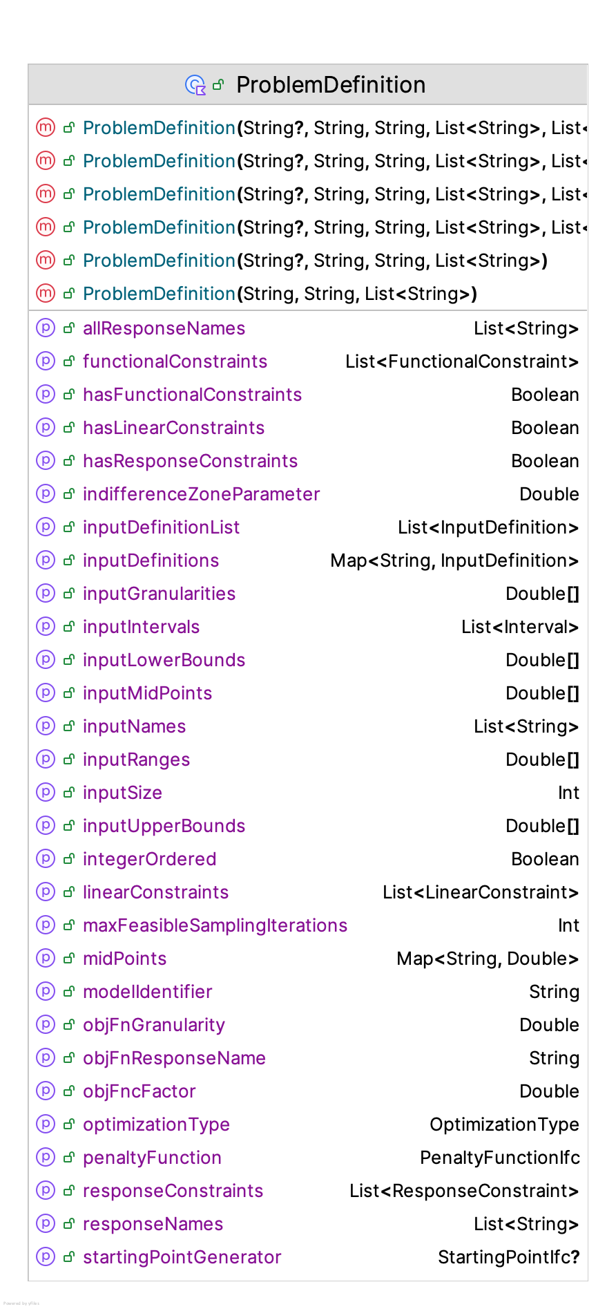
Figure 10.9: Problem Definition Properties

Let’s take a closer look at the constructor for the ProblemDefinition class.

class ProblemDefinition @JvmOverloads constructor(
    problemName: String? = null,
    val modelIdentifier: String,
    val objFnResponseName: String,
    inputNames: List<String>,
    responseNames: List<String> = emptyList(),
    val optimizationType: OptimizationType = OptimizationType.MINIMIZE,
    indifferenceZoneParameter: Double = 0.0,
    objFnGranularity: Double = 0.0
) : IdentityIfc by Identity(problemName)

The constructor requires a string modelIdentifier that represents a unique identifier for the model associated with the optimization problem. This identifier will be used to ensure that the simulation evaluation process connects the requests for simulation evaluations with the correct model.

We do not specify a functional form for the objective function, $G(\vec{x})$. Instead, the problem definition must specify a valid name for the simulation response variable that represents the objective function via the objFnResponseName property. Similarly, the problem definition requires the names of the response variables associated with the response constraints in the form of the responseNames list. The type of optimization problem must be specified. Finally, the list of strings, inputNames represents the named input (decision) variables related to the model. This list must not be empty. If the list has repeated elements, they are removed. We will discuss how to specify these names when an example is presented. The indifferenceZoneParameter parameter represents the smallest actual difference that is important to detect for the objective function response. This parameter can be used by solvers to determine if differences between solutions are considered practically significant. We will discuss the concept of granularity in Section 10.3.2.

Figure 10.10 presents the functions for the ProblemDefinition class. This functionality includes:

adding/defining/validating input variables
adding/defining linear constraints
adding/defining functional constraints
adding/defining response constraints
randomly generating feasible points in the input space
converting arrays of variables to valid input variables
checking for different feasibility conditions and computing constraint violations
specifying a penalty function for translating a constrained problem to an unconstrained problem
representing neighborhoods for the problem

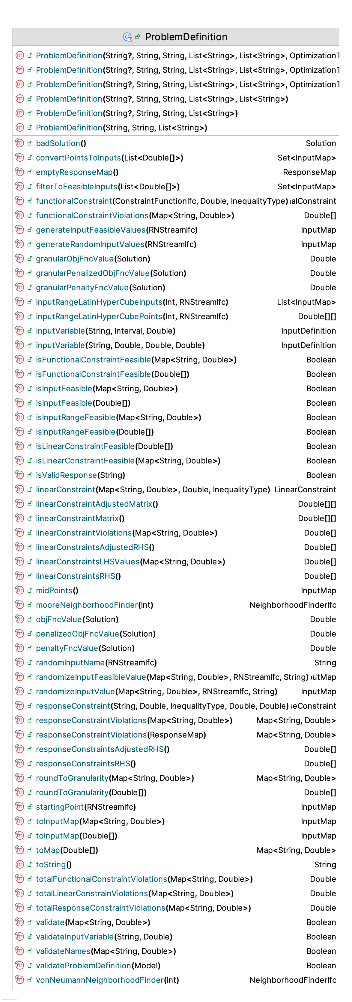
Figure 10.10: Problem Definition Properties

10.3.1 Specifying Penalty Functions

Many algorithms utilize penalty functions to address constraint violations within the search process. Penalty functions are a variation on the Lagrangian approach of converting a constrained optimization into an unconstrained optimization problem. Recall the standardized minimization representation:

\[ \min g(\vec{x}) = E[G(\vec{x})] \\ \sum_{i=1}^{|I|}a_{ij}x_i \leq b_j \quad \textrm{for} \quad j=1,\dots,|L|\\ f_{i} (\vec{x}) \leq c_{i} \quad \textrm{for} \quad i=1,\dots,|F|\\ E[R_{i}(\vec{x})] \leq r_i \quad \textrm{for} \quad i=1,\dots,|R|\\ l_i \leq x_i \leq u_i \quad \textrm{for} \quad i=1,\dots,|I|\\ \] We see that each constraint is presented as a less than or equal to constraint. Let’s call the left-hand side of any constraint, $LHS_k$, and the right-hand side $RHS_k$, where $k$ represents one of the linear, functional or response constraints. A violation of the constraint occurs if $LHS_k > RHS_k$. If this occurs, then we have a violation, and the amount of the violation is the difference, $LHS_k - RHS_k$. Let $v_k$ represent the violation associated with constraint $k$, where $v_k = \max(0, LHS_k - RHS_k)$. Let $K$ represent the total number of constraints. That is $K = |L| + |F| + |R|$. For the purposes of the penalty function, we ignore the lower and upper bound constraints. If you need to include a bound type constraint within the penalty function processing, then you can easily do that by using a linear constraint. There are many possible approaches to defining a penalty function. To facilitate different kinds of penalty functions, the ksl.simopt.problem package provides a PenaltyFunctionIfc interface.

fun interface PenaltyFunctionIfc {

    /**
     *  The penalty function.
     *  @param solution The solution for which the penalty is being computed.
     *  @param iterationCounter The current iteration count. The iteration associated
     *  with the solver's process.
     */
    fun penalty(solution: Solution, iterationCounter: Int): Double

}

The penalty function is a function of the solution and an iteration counter. The iteration counter represents the current iteration of the solver that produced the solution. Note that the PenalityFunctionIfc interface is a functional interface. Thus, Kotlin’s anonymous functions can be used to supply your own implementation of a penalty function.

The default penalty function has the following mathematical form. Define $M(k,\xi)$ as an increasing sequence in the form $M_0 k^\xi$, where $M_0 \in \mathbb{R}^+$ is called the initial penalty parameter and $\xi > 0$. This form of penalty function is suggest in (Park and Kim 2015). Let $l_v$, $f_v$, and $r_v$, represent the total violations associated with the linear, functional, and response constraints, respectively. Let $l_0$, $f_0$, and $r_0$ represent the initial penalty parameters for the linear, functional, and response constraints, respectively. Finally, let $t_v$ be the total penalized violations, $k$ be the iteration number, and $P(\vec{x},k)$ be the penalty as a function of the solution and iteration number.

\[ l_v = \sum_{k \in L} v_k \\ f_v = \sum_{k \in F} v_k \\ r_v = \sum_{k \in R} v_k \\ t_v = l_0*l_v + f_0*f_v * r_0*r_v\\ P(\vec{x},k) = k^\xi*t_v \] The optimization problem becomes:

\[ \min g(\vec{x}) = E[G(\vec{x})] + P(\vec{x},k)\\ \] The DefaultPenaltyFunction class implements these concepts. The default initial penalty values of $l_0$, $f_0$, and $r_0$ are set to 1000, and the default exponent, $\xi= 2$. In essence, the default penalty function penalizes the total violations and increases the penalty as the iteration number increases. Users can change these defaults or provide there own initial penalty values or exponent value. The ProblemDefinition class facilitates the computation of each type of violation, individually for each constraint and in total via the functions:

linearConstraintViolations(inputs: Map<String, Double>): DoubleArray
totalLinearConstrainViolations(inputs: Map<String, Double>): Double
functionalConstraintViolations(inputs: Map<String, Double>): DoubleArray
totalFunctionalConstraintViolations(inputs: Map<String, Double>): Double

Users can use these functions to define their own penalty function forms.

10.3.2 Defining Input Variables

For optimization problems, the decision variables are the key quantities that need to be determined. For a ProblemDefinition instance, the InputDefinition class, illustrated in Figure 10.11 is used to define the decision variables.

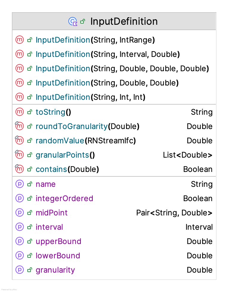
Figure 10.11: The InputDefinition Class

The constructor for defining inputs is as follows:

class InputDefinition @JvmOverloads constructor(
    val name: String,
    val lowerBound: Double,
    val upperBound: Double,
    granularity: Double = 0.0
)

The user provides the name of the input and its bounds. The name must match one of the input names within the problem definition instance.

Finally, there is the granularity parameter. The specified granularity indicates the acceptable precision for the variable’s value with respect to decision-making. If the granularity is 0 then no rounding will be applied when evaluating the variable. Granularity defines the level of precision for an input variable to which the problem will be solved. Setting granularity to 0, the default, means that the solver will attempt to find a solution to the level of machine precision. For any positive granularity value, the solution will be found to some multiple of that granularity. As a special case, setting granularity to 1 implies an integer-ordered input variable. The specification of granularity reflects a reality for the decision maker that there is a level of precision beyond which it is not practical to implement a solution.

Granularity represents the finest division of the measurement scale. For example, a 12-inch rule that has inches divided into 4 quarters has a granularity of 1/4 or 0.25. The granularity parameter specifies the degree of this precision so that a function can be applied which rounds the supplied value to the nearest multiple of the granularity. Suppose, we had a quarter inch granularity, the rounding process would round 3.1459 to 3.25 because 3.25 is the nearest multiple of the granularity of (0.25). For the case of 3.0459 with a granularity of 0.25, the value of 3.0459 would be rounded to 3.0. Thus, with a quarter inch granularity we can only have values that are multiples of 0.25. In essence, this permits a discretization of a continuous variable to points that are realistic with respect to the measurement scale associated with the variable. Thus, continuous variables can be handled as discrete variables if necessary. This functionality recognizes that any variable represented on a digital computer is a discrete representation (even to machine precision). For many realistic problems, from a practical standpoint, we cannot implement decision variables beyond some level of granularity.

If an input variable is defined with a granularity of 1.0, then it is considered integer-ordered. If an optimization problem has only integer-ordered decision variables, then the problem is considered integer-ordered. Some solvers are constructed to specifically handle this kind of problem. The R-SPLINE solver discussed in (Wang et al. 2013) is an integer-ordered solver and has been implemented within the KSL.

10.3.3 Linear and Functional Constraints

The specification of constraints is similar to defining input variables. The ProblemDefinition class provides functions that allow the specification of each type of constraint: linear, functional, and response. The LinearConstraint class indicates how to compute a linear constraint. Figure 10.12 presents the ConstraintIfc interface with two implementations in the LinearConstraint and FunctionalConstraint classes.

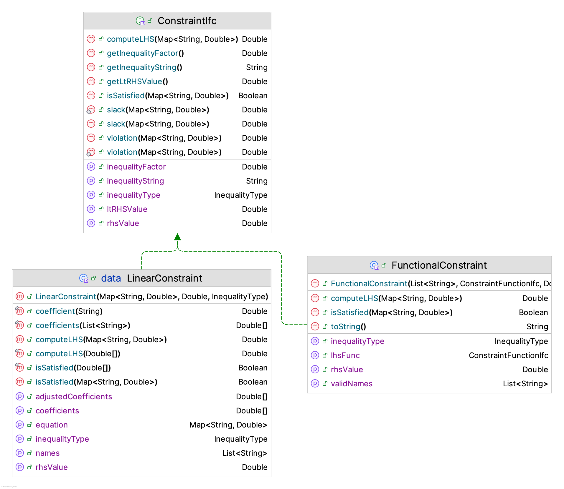
Figure 10.12: Deterministic Constraints

The LinearConstraint class takes in a map that provides the coefficient $a_i$ associated with each decision variable $x_i$. Because of the linear form of the equation, this representation is sufficient to define the linear equation. In addition, the right-hand side variable $b_j$ and the form of the inequality is specified. The class will translate a greater than constraint to the mathematically equivalent less than constraint.

data class LinearConstraint(
    val equation: Map<String, Double>,
    override var rhsValue: Double = 0.0,
    override val inequalityType: InequalityType = InequalityType.LESS_THAN
) : ConstraintIfc

As noted in Figure 10.12, deterministic constraints can compute the left-hand side of the constraint and compare it with the right-hand side to determine if the constraint is satisfied, whether there is slack in the constraint, and the amount of the constraint’s violation.

As shown in the FunctionalConstraint constructor, the constraint is defined as a function of the input parameters.

class FunctionalConstraint(
    validNames: List<String>,
    val lhsFunc: ConstraintFunctionIfc,
    override val rhsValue: Double = 0.0,
    override val inequalityType: InequalityType = InequalityType.LESS_THAN
) : ConstraintIfc {

The ConstraintFunctionIfc interface is a functional interface. It simply takes in a map containing the named input variables and their values and returns the left-hand side of the constraint. Thus, the user can specify any functional form by implementing this interface.

fun interface ConstraintFunctionIfc {

    fun lhs(inputs: Map<String, Double>): Double

}

10.3.4 Response Constraints

The final type of constraint is the response constraint. Response constraints are different from deterministic constraints because these constraints rely on the execution of the simulation model for the observation of their values. These are very difficult constraints within a mathematical programming context. Figure 10.13 provides the KSL representation for modeling response constraints.

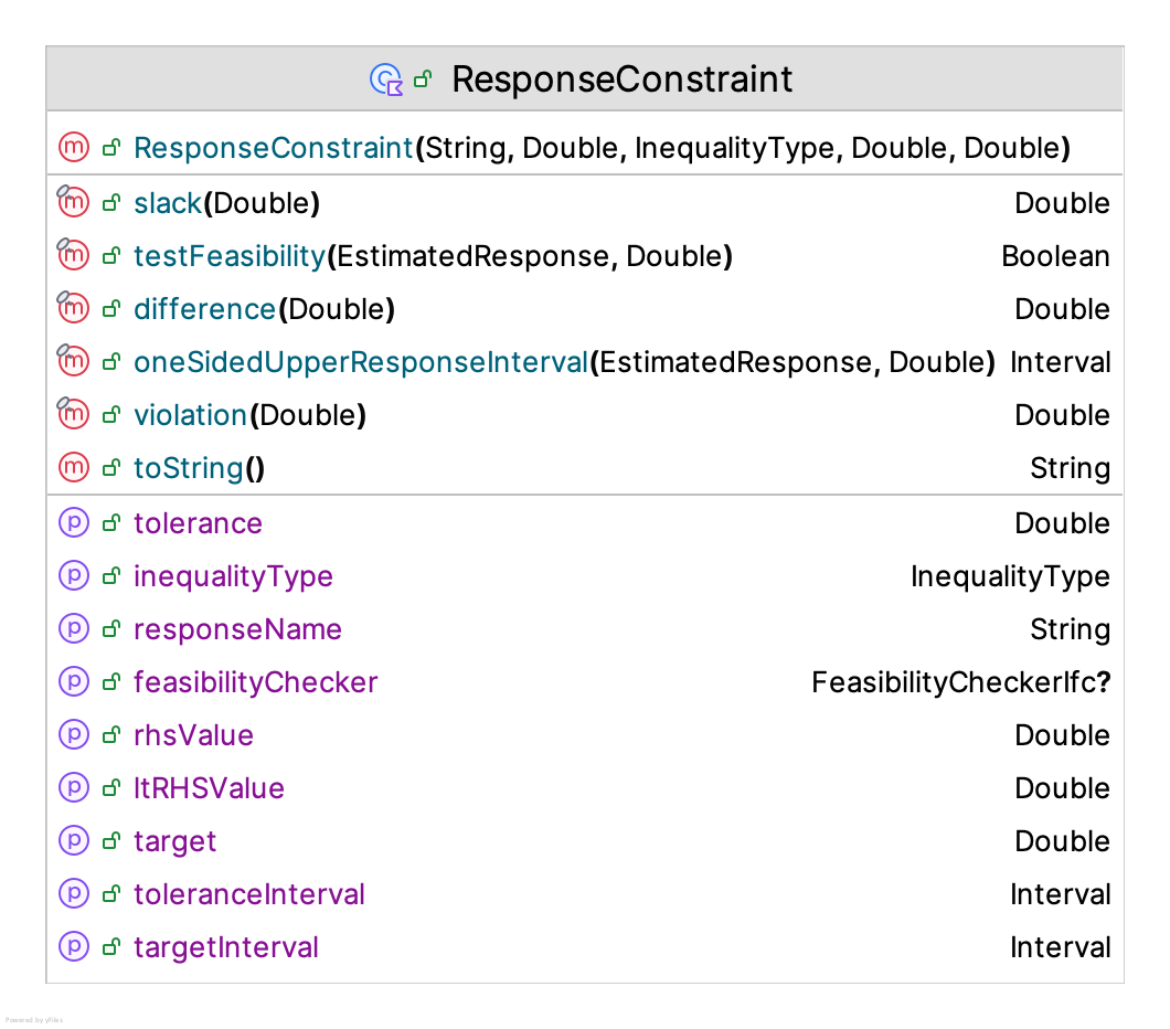
Figure 10.13: Response Constraints

A response constraint requires the name of a valid simulation response variable, the right-hand side value, and the type of inequality. In addition, some solvers may utilize information about a constraint in the form of a target and a tolerance. The target parameter is used by some algorithms to serve as a cut-off point between desirable and unacceptable solutions with respect to the constraint. The tolerance parameter is used by some algorithms to specify how much the decision maker is willing to be off from the target and is conceptually similar to an indifference parameter.

class ResponseConstraint(
    val responseName: String,
    val rhsValue: Double,
    val inequalityType: InequalityType = InequalityType.LESS_THAN,
    val target: Double = 0.0,
    val tolerance: Double = 0.0
) {

Response constraints will also compute the slack and violation amounts. The default implementation is to not take into account randomness in these calculations. In essence, this treats the estimated response value as “deterministic” when computing the violation. Recognizing that feasibility checking may be more complex with these stochastic constraints, the ResponseConstraint class permits the user to supply an instance of a the FeasibilityCheckerIfc interface.

fun interface FeasibilityCheckerIfc {

    fun isFeasible(
        responseConstraint: ResponseConstraint,
        estimatedResponse: EstimatedResponse,
        confidenceLevel: Double
    ): Boolean
}

The FeasibilityCheckerIfc interface allows for the checking of feasibility based on some statistical confidence. If the user supplies an instance of this interface, then it will be used when testing for feasibility for a response constraint. Now, let’s take a look at an example to illustrate how to specify a problem.

10.3.5 Setting Up a Problem Definition

Example 10.1 (Reorder Point, Reorder Quantity Inventory Model) An inventory manager is interested in understanding the cost and service trade-offs related to the inventory management of computer printers. Suppose customer demand occurs according to a Poisson process at a rate of 3.6 units per month and the lead time is 0.5 months. The manager has estimated that the holding cost for the item is approximately $0.25 per unit per month. In addition, when a back-order occurs, the estimate cost will be $1.75 per unit per month. Every time that an order is placed, it costs approximately $0.15 to prepare and process the order. The inventory manager wants to find the optimal setting for the reorder point and the reorder quantity with respect to the total ordering and holding cost while ensuring a fill rate of at least 0.95. Set up a KSL simulation optimization problem for this situation.

This is Example 7.9 from Chapter 7. To prepare to use the implemented model from Example 7.9, we need to ensure that controls are defined for the input variables and to note the names of the responses involved in the problem. The two decision variables are the reorder point and the reorder quantity. Within the RQInventory class, we have the following defined controls:

    @set:KSLControl(
        controlType = ControlType.INTEGER,
        lowerBound = 0.0
    )
    var initialReorderPoint: Int
        get() = myInitialReorderPt
        set(value) {
            setInitialPolicyParameters(value, myInitialReorderQty)
        }

    @set:KSLControl(
        controlType = ControlType.INTEGER,
        lowerBound = 1.0
    )
    var initialReorderQty: Int
        get() = myInitialReorderQty
        set(value) {
            setInitialPolicyParameters(myInitialReorderPt, value)
        }

Recall from Section 5.8.1 of Chapter 5 that the name of the control will be the model element’s name concatenated with the name of the property separated by a “dot”. In the RQInventorySystem class definition, we see that the instances of inventory use the name supplied for the parent with the string “Item” as shown in the following code.

private val inventory: RQInventory = RQInventory(
    this, reorderPt, reorderQty, replenisher = Warehouse(), name = "${this.name}:Item"
)

Thus, the names of the two controls will be the strings:

“Inventory:Item.initialReorderQty”
“Inventory:Item.initialReorderPoint”

The fill rate and total ordering and holding cost responses have similar naming conventions resulting in these strings:

“Inventory:Item:FillRate”
“Inventory:Item:OrderingAndHoldingCost”

These names are essential for constructing the problem definition. Section 5.8.1 also describes how to get the names of all controls within a model.

Finally, we need to know the model identifier. By default, this will be the assigned the name of the model, but in general it is user assignable. The basic code for building the reorder point, reorder quantity inventory model is as follows:

val reorderQty: Int = 2
val reorderPoint: Int = 1
val model = Model("RQInventoryModel")
val rqModel = RQInventorySystem(model, reorderPoint, reorderQty, "Inventory")
rqModel.initialOnHand = 0
rqModel.demandGenerator.initialTimeBtwEvents = ExponentialRV(1.0 / 3.6)
rqModel.leadTime.initialRandomSource = ConstantRV(0.5)
model.lengthOfReplication = 20000.0
model.lengthOfReplicationWarmUp = 10000.0
model.numberOfReplications = 40

Thus, the model identifier will be the string “RQInventoryModel”. Now, the code for constructing the problem definition can be completed.

val problemDefinition = ProblemDefinition(
    problemName = "InventoryProblem",
    modelIdentifier = "RQInventoryModel",
    objFnResponseName = "Inventory:Item:OrderingAndHoldingCost",
    inputNames = listOf("Inventory:Item.initialReorderQty", "Inventory:Item.initialReorderPoint"),
    responseNames = listOf("Inventory:Item:FillRate")
)
problemDefinition.inputVariable(
    name = "Inventory:Item.initialReorderQty",
    interval = Interval(1.0, 100.0),
    granularity = 1.0
)
problemDefinition.inputVariable(
    name = "Inventory:Item.initialReorderPoint",
    interval = Interval(1.0, 100.0),
    granularity = 1.0
)
problemDefinition.responseConstraint(
    name = "Inventory:Item:FillRate",
    rhsValue = 0.95,
    inequalityType = InequalityType.GREATER_THAN
)

The constructor uses a user assignable name for the problem, the model identifier, the name of the response for the objective function, the names of the input (decision) variables, and the names of the responses. Note that the type of optimization was not specified. Thus, the type is minimization by default. Then, the two input variables representing the initial reorder point and initial reorder quantity are defined over search intervals. Notice that the granularity is set to 1.0, which indicates that this is an integer-ordered (discrete) problem. Finally, the fill rate constraint is added to indicate that desired solutions need to have the fill-rate response greater than 95 percent. The problem definition instance will be required when setting up the solver and the simulation evaluation process.

G References

Park, Chuljin, and Seong-Hee Kim. 2015. “Penalty Function with Memory for Discrete Optimization via Simulation with Stochastic Constraints.” Operations Research 63 (5): 1195–212. https://doi.org/10.1287/opre.2015.1417.

Wang, Honggang, Raghu Pasupathy, and Bruce W. Schmeiser. 2013. “Integer-Ordered Simulation Optimization Using R-SPLINE: Retrospective Search with Piecewise-Linear Interpolation and Neighborhood Enumeration.” ACM Transactions on Modeling and Computer Simulation (TOMACS) 23 (3): 17–24. https://doi.org/10.1145/2499913.2499916.