D.9 Experimental Design Utilities
As discussed in Section 5.8.3 of Chapter 5 when analyzing a situation using simulation, we must often simulate a model many times. This initiates the need to be efficient and effective when running many scenarios. Experimental design concepts can assist with ensuring an efficient and effective approach to experimenting with a simulation model.
An experiment is a data collection procedure that occurs under controlled conditions to identify and understand the relationships between variables. A computer simulation experiment is an experiment executed (virtually) on a computer using a simulation model. The simulation model is a proxy representation for the actual physical system. When you run a simulation model, you are performing an experiment. Computer simulation is experimentation on a computer. An experimental design is a detailed plan for collecting and using data to understand the relationships between variables. An experimental design describes how to execute the experiment. For a computer simulation, an experimental design details the settings for the model’s inputs and the specification of the desired outputs. Experimental design is an iterative process. Don’t expect to get the plan perfect the first time or without some preliminary ad-hoc experimentation. The goal of experimental design is to be able to understand the relationships between the variables in the most efficient and effective manner possible.
Factors are the attributes of the model (parameters and/or input variables) that may be changed (or controlled) in a simulation experiment. Factors are the parameters/inputs that are of interest during experimentation. The factor levels are the set of possible values that factors are changed to (set at) for an experimental run. These are sometimes called treatments in physical experiments, but generally not so for computer experiments. For example, if the reorder quantity is a factor, the the levels might be (5, 20, 50) units. The levels are the settings that can be used for the factor. A design point is the specification of an instance of factor settings that will result in observations of the response. An experimental run (or run) is the execution of an experimental design point resulting in a single observation of the output variables. In experimental design, an experimental run is often called a replicate. In the simulation context, it is often referred to as a replication. An experimental design can be thought of as the set of design points and the specification of how many replications are required for each point.
The KSL provides functionality to define and run experiments based on experimental design contexts. We start with being able to represent factors. Figure 10.1 presents the class diagram for the Factor class. Factors have a name and a specification of the levels for the factors.
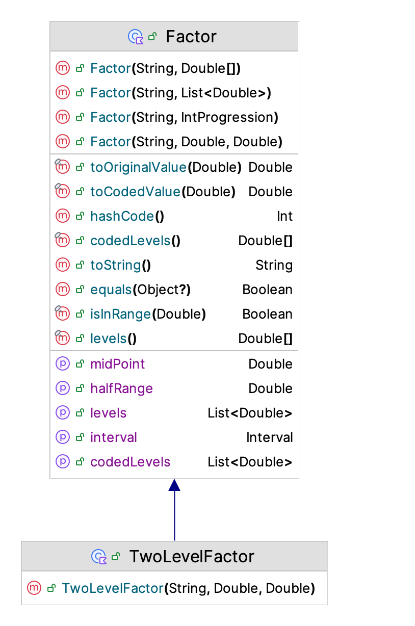
Figure 10.1: KSL Factors
When setting up an experimental design, the regressors (factors) are often coded in such a manner to facilitate the interpretation of the model coefficients. Quite often they are scaled to a range of values between -1 and 1, or between 0 and 1. Within the KSL, the levels of the factors should be supplied via their uncoded values. The KSL Factor class can perform the translation to and from the coded and uncoded design space.
Suppose we have non-standardized factor \(p\) and denoted as \(w_p\). Suppose \(w_p\) ranges between its lowest value, \(l_p\) and its highest value \(u_p\). That is \(w_p\) is in the interval, \(w_p \in [l_p,u_p]\). For example, suppose \(w_p\) is the mean of the service time distribution and \(w_p\) has levels \([5,10,15,20,25]\). Thus, \(l_p = 5\) and \(u_p = 25\)
- Let \(h_p\) be the half-range, where \(h_p = (u_p - l_p)/2\). The half-range measures the spread of the factor.
- Let \(m_p\) be the mid-point of the range, where \(m_p = (u_p + l_p)/2\).
A standard approach is to the code the factor as:
\[ x_{ip}=\frac{w_{ip} - m_{p}}{h_p} \]
For example, suppose \(w_{ip} \in \{5,10,15,20,25\}\). Thus \(h_p = (25 - 5)/2 = 10\) and \(m_p = (25 + 5)/2 = 15\). Thus, we have \(x_{ip} \in \{-1,\frac{-1}{2},0,\frac{1}{2},1\}\). Notice that for a factor with two levels this always results in a coding of \(\pm 1\). Low is coded to \(-1\) and high is coded to \(+1\).
The following illustrates the creation of two factors, one with 3 levels and another with 2 levels.
    val f1 = Factor("A", doubleArrayOf(1.0, 2.0, 3.0, 4.0))
    val f2 = Factor("B", doubleArrayOf(5.0, 9.0))
    val factors = setOf(f1, f2)
Once we have defined factors for the experiment, we can proceed with defining an experimental design. The KSL supports factorial designs, two level factorial designs, central composite designs, and general experimental designs. Figure 10.2 presents the major classes and interfaces related to KSL experiments.
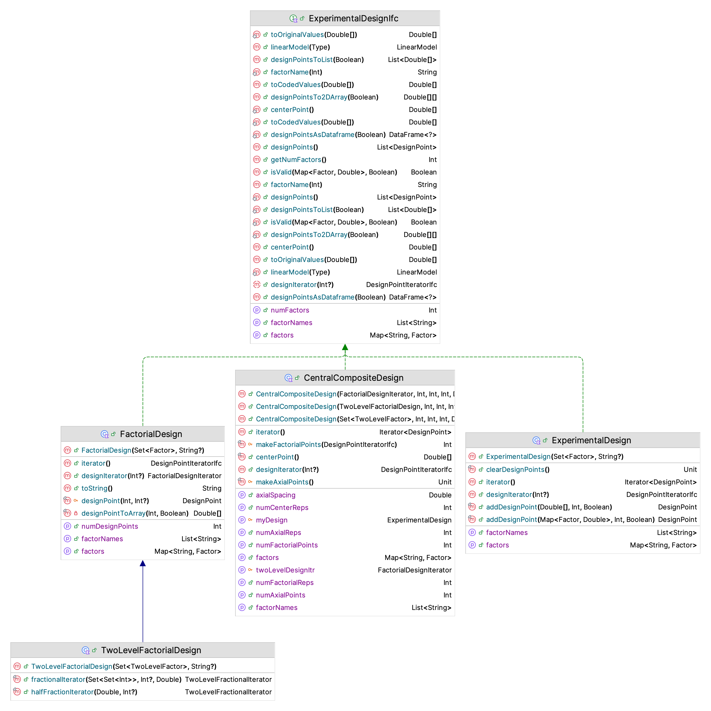
Figure 10.2: KSL Experimental Design Classes
The first important item to note is the use of the ExperimentalDesignIfc interface. The experimental designs supported by the KSL all implement this interface. The ExperimentalDesignIfc interface provides functionality that allows the design points in the design to be specified and iterated. To create an experimental design, you must specify the set of factors, or as in the case of a composite design, the starting factorial design.
The following code illustrates how to create a factorial design and will print out the design points.
    val f1 = Factor("A", doubleArrayOf(1.0, 2.0, 3.0, 4.0))
    val f2 = Factor("B", doubleArrayOf(5.0, 9.0))
    val factors = setOf(f1, f2)
    val fd = FactorialDesign(factors)
    println(fd)
    println()
    println("Factorial Design as Data Frame")
    println(fd.designPointsAsDataframe())
    println()
    println("Coded Factorial Design as Data Frame")
    println(fd.designPointsAsDataframe(true))
    println()
There are eight design points in this design because we have factor A with 4 levels and factor B with 2 levels, resulting in \(4 \times 2 = 8\) design points.
FactorialDesign
name: ID_3
number of design points: 8
Factors
Factor: A
Levels = 1.0,2.0,3.0,4.0
halfRange = 1.5
midPoint = 2.5
Coded Levels = -1.0,-0.3333333333333333,0.3333333333333333,1.0

Factor: B
Levels = 5.0,9.0
halfRange = 2.0
midPoint = 7.0
Coded Levels = -1.0,1.0

Factorial Design as Data Frame
     A   B
 0 1.0 5.0
 1 1.0 9.0
 2 2.0 5.0
 3 2.0 9.0
 4 3.0 5.0
 5 3.0 9.0
 6 4.0 5.0
 7 4.0 9.0

 Coded Factorial Design as Data Frame
           A    B
 0 -1.000000 -1.0
 1 -1.000000  1.0
 2 -0.333333 -1.0
 3 -0.333333  1.0
 4  0.333333 -1.0
 5  0.333333  1.0
 6  1.000000 -1.0
 7  1.000000  1.0
A two-level factorial design is a special case of the more general factorial design where factors can have more than two levels. For two-level factorial designs, the KSL provides the TwoLevelFactorialDesign class. The following code illustrates how to create a two-level factorial design.
    val design = TwoLevelFactorialDesign(
        setOf(
            TwoLevelFactor("A", 5.0, 15.0),
            TwoLevelFactor("B", 2.0, 11.0),
            TwoLevelFactor("C", 6.0, 10.0),
            TwoLevelFactor("D", 3.0, 9.0),
        )
    )
    val fdf = design.designPointsAsDataframe()
    println("Full design points")
    fdf.print(rowsLimit = 36)
    println("Coded full design points")
    design.designPointsAsDataframe(true).print(rowsLimit = 36)
    println()
Note that for this design, you need to define the factors using the TwoLevelFactor class, which restricts the levels to only two values. Since there are only two levels, the coded values are (-1) and (+1).
Once you have a full two-level factorial design, you may want to only simulate a portion of the design. A fractional factorial design is an experimental design that specifies some fraction of the full factorial combination of design points. The most commonly specified fractional designs are one-half fraction of \(2^k\) designs. A \(\frac{1}{2}\) fraction of a \(2^k\) design has \(2^{k-1} = \frac{1}{2}2^k\) runs and is called a \(2^{k-1}\) fractional factorial design. In the context of \(2^k\) designs, we may have larger fractions, i.e. \(2^{k-p}\) designs, where \(p\ge 1\). Running a fraction of the design points reduces the number of runs but also limits what models can be estimated.
Using a \(\frac{1}{2}\) fraction creates two sets of runs. Below the rows have been rearranged so that column (123) starts with \(+1\) for the first half-fraction. A \(2^{3-1}\) fractional factorial design has \(2^2 = 4\) runs. Running the rows with \(+1\) of column (123), would be running the first (positive) \(\frac{1}{2}\) fraction of the design.
\[ \begin{array}{|c|c|c|c|c|c|c|c|c|} \hline I & (1) & (2) & (3) & (12) & (13) & (23) & (123) & Fraction\\ \hline +1 & +1 & -1 & -1 & -1 & -1 & +1 & +1 & Positive \\ \hline +1 & -1 & +1 & -1 & -1 & +1 & -1 & +1 & Positive \\ \hline +1 & -1 & -1 & +1 & +1 & -1 & -1 & +1 & Positive \\ \hline +1 & +1 & +1 & +1 & +1 & +1 & +1 & +1 & Positive \\ \hline +1 & +1 & +1 & -1 & +1 & -1 & -1 & -1 & Negative \\ \hline +1 & +1 & -1 & +1 & -1 & +1 & -1 & -1 & Negative \\ \hline +1 & -1 & +1 & +1 & -1 & -1 & +1 & -1 & Negative \\ \hline +1 & -1 & -1 & -1 & +1 & +1 & +1 & -1 & Negative \\ \hline \end{array} \]
We can specify fractional designs within the KSL by requesting an iterator from the full two-level design that contains the desired portion of the design. This can be accomplished with the halfFractionIterator() function or the fractionalIterator() function. The following code illustrates how to access these iterators.
    // create the full design
    val design = TwoLevelFactorialDesign(
        setOf(
            TwoLevelFactor("A", 5.0, 15.0),
            TwoLevelFactor("B", 2.0, 11.0),
            TwoLevelFactor("C", 6.0, 10.0),
            TwoLevelFactor("D", 3.0, 9.0),
            TwoLevelFactor("E", 4.0, 16.0)
        )
    )
    println("Positive half-fraction")
    val hitr = design.halfFractionIterator()
    // convert iterator to data frame for display
    hitr.asSequence().toList().toDataFrame(coded = true).print(rowsLimit = 36)
    println()
    // This is a resolution III 2^(5-2) design
    // This design can be found here: https://www.itl.nist.gov/div898/handbook/pri/section3/eqns/2to5m2.txt
    // Specify a design relation as a set of sets.
    // The sets are the columns of the design that define the associated generator
    val relation = setOf(setOf(1, 2, 4), setOf(1, 3, 5), setOf(2, 3, 4, 5))
    val itr = design.fractionalIterator(relation)
    println("number of factors = ${itr.numFactors}")
    println("number of points = ${itr.numPoints}")
    println("fraction (p) = ${itr.fraction}")
    val dPoints = itr.asSequence().toList()
    val df = dPoints.toDataFrame(coded = true)
    println("Fractional design points")
    df.print(rowsLimit = 36)
First the full factorial design is constructed. The halfFractionIterator() function has the following signature. The first parameter should be (+1.0) to get the positive half-fraction, or (-1.0) to get the negative half-fraction.
    /**
     *  @param half indicates the half-fraction to iterate. 1.0 indicates the positive
     *  half-fraction and -1.0 the negative half-fraction. The default is 1.0
     *  @param numReps the number of replications for the design points.
     *  Must be greater or equal to 1. If null, then the current value for the
     *  number of replications of each design point is used. Null is the default.
     */
    fun halfFractionIterator(half: Double = 1.0, numReps: Int? = null): TwoLevelFractionalIterator
The results of the half-fraction code are as follows. Notice that there are only 16 (of the 32) design points.
Positive half-fraction
       A    B    C    D    E
  0 -1.0 -1.0 -1.0 -1.0  1.0
  1 -1.0 -1.0 -1.0  1.0 -1.0
  2 -1.0 -1.0  1.0 -1.0 -1.0
  3 -1.0 -1.0  1.0  1.0  1.0
  4 -1.0  1.0 -1.0 -1.0 -1.0
  5 -1.0  1.0 -1.0  1.0  1.0
  6 -1.0  1.0  1.0 -1.0  1.0
  7 -1.0  1.0  1.0  1.0 -1.0
  8  1.0 -1.0 -1.0 -1.0 -1.0
  9  1.0 -1.0 -1.0  1.0  1.0
 10  1.0 -1.0  1.0 -1.0  1.0
 11  1.0 -1.0  1.0  1.0 -1.0
 12  1.0  1.0 -1.0 -1.0  1.0
 13  1.0  1.0 -1.0  1.0 -1.0
 14  1.0  1.0  1.0 -1.0 -1.0
 15  1.0  1.0  1.0  1.0  1.0
The fractionalIterator() function is more complicated. It’s signature is as follows.
    fun fractionalIterator(
        relation: Set<Set<Int>>,
        numReps: Int? = null,
        sign: Double = 1.0
    ): TwoLevelFractionalIterator {
        return TwoLevelFractionalIterator(relation, numReps, sign)
    }
This iterator should present each design point in the associated fractional design until all points in the fractional design have been presented. The iterator checks if the coded values of the design point are in the defining relation specified by the factor numbers stored in the relation set. Suppose the designing relation is I = 124 = 135 = 2345. Then relation specification is setOf(setOf(1,2,4), setOf(1,3,5), setOf(2,3,4,5)). The values in the words must be valid factor indices. That is, if a design has 5 factors, then the indices must be in the set (1,2,3,4,5), with 1 referencing the first factor, 2 the 2nd, etc.
To learn more about fractional designs and design generators, we refer the interested reader to the fractional factorial design section of the NIST Engineering Statistics Handbook.
The resulting design points for the \(2^{5-2}\) resolution III design are as follows. Notice that there are only 8 design points in this resolution III design.
number of factors = 5
number of points = 8
fraction (p) = 2
Fractional design points
      A    B    C    D    E
 0 -1.0 -1.0 -1.0  1.0  1.0
 1 -1.0 -1.0  1.0  1.0 -1.0
 2 -1.0  1.0 -1.0 -1.0  1.0
 3 -1.0  1.0  1.0 -1.0 -1.0
 4  1.0 -1.0 -1.0 -1.0 -1.0
 5  1.0 -1.0  1.0 -1.0  1.0
 6  1.0  1.0 -1.0  1.0 -1.0
 7  1.0  1.0  1.0  1.0  1.0
As illustrated for the fractional design case, an iterator over design points is an essential component of how the KSL implements its experimental design functionality. Figure 10.3 illustrates the basic functionality of a design point iterator.
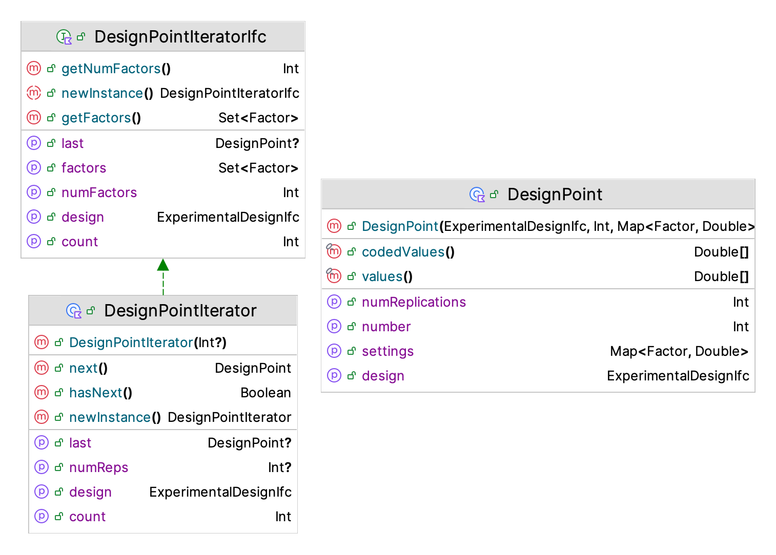
Figure 10.3: KSL Design Point Iterator Classes
There are a couple of items of note. First, a design point knows the number of replications it will require and has access to the factors and to the associated design. The design point can provide coded and uncoded values. The design point iterator also has access to the factors, the design, and can move through the design points. This functionality is essential for how the DesignedExperiment class operates. The purpose of the DesignedExperiment class is to facilitate the simulation of an experimental design. The DesignedExperiment class causes each design point in its supplied design to be simulated for the specified number of replications.
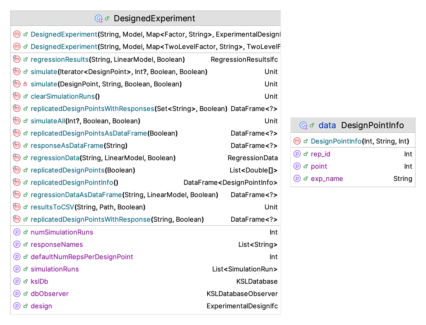
Figure 10.4: KSL DesignedExperiment Class
Figure 10.4 illustrates the KSL’s DesignedExperiment class. The signature of its constructor is as follows.
class DesignedExperiment(
    name: String,
    private val model: Model,
    private val factorSettings: Map<Factor, String>,
    val design: ExperimentalDesignIfc,
    val kslDb: KSLDatabase = KSLDatabase("${name}.db".replace(" ", "_"),
        model.outputDirectory.dbDir)
) : Identity(name) {
Notice that the constructor requires a name for the experiment, the model that will be exercised, the factorial settings, and the experimental design. The factor settings are specified by using controls or random variable parameter settings. The following code sets up a three factor, two level factorial design and simulates the design points.
    val fA = Factor("Server", doubleArrayOf(1.0, 2.0, 3.0))
    val fB = Factor("MeanST", doubleArrayOf(0.6, 0.7))
    val fC = Factor("MeanTBA", doubleArrayOf(1.0, 5.0))
    val factors = mapOf(
        fA to "MM1Q.numServers",
        fB to "MM1_Test:ServiceTime.mean",
        fC to "MM1_Test:TBA.mean"
    )
    val m = Model("DesignedExperimentDemo")
    m.numberOfReplications = 15
    m.lengthOfReplication = 10000.0
    m.lengthOfReplicationWarmUp = 5000.0
    val ggc = GIGcQueue(m, 1, name = "MM1Q")

    val fd = FactorialDesign(factors.keys)
    val de = DesignedExperiment("FactorDesignTest", m, factors, fd)

    println("Design points being simulated")
    fd.designPointsAsDataframe().print(rowsLimit = 36)
    println()
    de.simulateAll(numRepsPerDesignPoint = 3)
    println("Simulation of the design is completed")
    de.resultsToCSV()
Notice that you can specify how many times each design point is replicated when simulating the design. This class works in a very similar manner as that described in Section 5.8.3 of Chapter 5 for running multiple scenarios. The DesignedExperiment class captures the results from the simulation runs to a database, which can be found in the dbDir directory associated with the model being simulated. The DesignedExperiment class also provides multiple ways to capture the design and its results, especially in the form of a data frame. The results can be easily exported to a CSV file for further analysis by your favorite statistical software.
    println("Replicated design points")
    de.replicatedDesignPointsAsDataFrame().print(rowsLimit = 36)
    println()
    println("Responses as a data frame")
    de.responseAsDataFrame("System Time").print(rowsLimit = 36)
    println()
    de.replicatedDesignPointsWithResponse("System Time").print(rowsLimit = 36)
    println()
    de.replicatedDesignPointsWithResponses().print(rowsLimit = 36)
    println()
    de.replicatedDesignPointsWithResponses(coded = true).print(rowsLimit = 36)
Notice that the results for all responses, an individual response, and the design points (coded or uncoded) are readily available for further analysis.
This final example illustrates how the results from a designed experiment can be analyzed using linear regression. The following code creates a model for a reorder level, reorder quantity inventory model. Details of this model can be found in Section 7.3.2 of Chapter 7. The following code creates the KSL discrete-event simulation model.
    val m = Model("ResponseSurfaceDemo")
    val rqModel = RQInventorySystem(m, name = "RQInventory")
    rqModel.costPerOrder = 0.15 //$ per order
    rqModel.unitHoldingCost = 0.25 //$ per unit per month
    rqModel.unitBackorderCost = 1.75 //$ per unit per month
    rqModel.initialReorderPoint = 2
    rqModel.initialReorderQty = 3
    rqModel.initialOnHand = rqModel.initialReorderPoint + rqModel.initialReorderQty
    rqModel.timeBetweenDemand.initialRandomSource = ExponentialRV(1.0 / 3.6)
    rqModel.leadTime.initialRandomSource = ConstantRV(0.5)
    m.lengthOfReplication = 72.0
    m.lengthOfReplicationWarmUp = 12.0
    m.numberOfReplications = 30
In the following code, we setup two factors, one for the reorder level and one for the reorder quantity. Then, we specify the factorial design.
    val r = TwoLevelFactor("ReorderLevel", low = 1.0, high = 5.0)
    println(r)
    val q = TwoLevelFactor("ReorderQty", low = 1.0, high = 7.0)
    println(q)
    println()
    val design = TwoLevelFactorialDesign(setOf(r, q))
    println("Design points being simulated")
    val df = design.designPointsAsDataframe()
    df.print(rowsLimit = 36)
Finally, we specify the settings of the factors using controls. See Section 5.8.1 for more on controls. Then, we specify the designed experiment and simulate all of the design points. Each design point is replicated 20 times.
    val settings = mapOf(
        r to "RQInventory:Item.initialReorderPoint",
        q to "RQInventory:Item.initialReorderQty",
    )
    val de = DesignedExperiment("R-Q Inventory Experiment", m, settings, design)
    de.simulateAll(numRepsPerDesignPoint = 20)
    println("Simulation of the design is completed")
After running the design, we can access the design points and the results. Then, we can run a linear regression based on the results stored in the data frame. Figure 10.5 presents the functions and properties of the KSL LinearModel class.
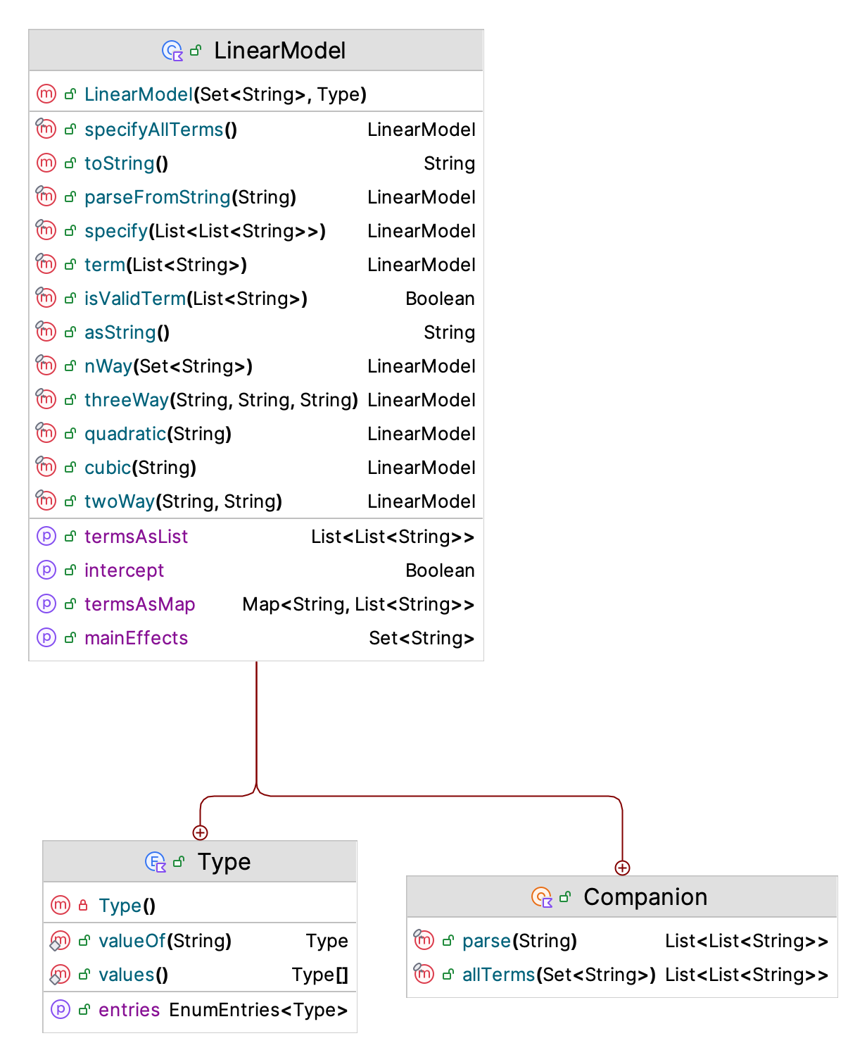
Figure 10.5: KSL LinearModel Class
The KSL LinearModel class provides the ability to specify a linear model (for use in regression and design of experiments). This is only a string specification of the linear model. The terms are specified by the names of the factors. As an example, consider a model with three factors, “A”, “B”, “C”, with full model = “A B C A*B A*C B*C A*B*C”. The full regression model for this situation is:
\[ y = \beta_0 + \beta_1 x_1 + \beta_2 x_2 + \beta_3 x_3 + \beta_{12} x_1 x_2 + \beta_{13} x_1 x_3 + \beta_{23} x_2 x_3 + \beta_{123} x_1 x_2 x_3 + \epsilon \]
To specify this model using the KSL LinearModel class, we use the following.
The KSL LinearModel class has functions that allow you to build the terms of the model. In addition, you can parse a string representation, such as “A B C A*B A*C B*C A*B*C”, to build the model. Let’s take a look at the code for specifying the linear model for the reorder point, reorder quantity model.
    val resultsDf = de.replicatedDesignPointsWithResponse("RQInventory:Item:TotalCost", coded = true)
    resultsDf.print(rowsLimit = 80)
    println()
    val lm = design.linearModel(type = LinearModel.Type.AllTerms)
    println(lm.asString())
    println()
    val lmDF = resultsDf.addColumnsFor(lm)
    lmDF.print(rowsLimit = 80)
    val regressionResults = de.regressionResults("RQInventory:Item:TotalCost", lm)
    println()
    println(regressionResults)
    regressionResults.showResultsInBrowser()
The design points and the responses are extracted from the designed experiment into a data frame with the following line of code.
Then, an instance of the LinearModel class is created based on all the terms available in the model.
This results in the output representing the linear model.
ReorderQty ReorderLevel ReorderLevel*ReorderQtyThis is essentially the following linear regression model.
\[ y = \beta_0 + \beta_1 x_1 + \beta_2 x_2 + \beta_{12} x_1 x_2 + \epsilon \]
To illustrate how to use the linear model to setup the data frame to perform the regression analysis we can use the following line of code.
In this case, the product term “ReorderLevel*ReorderQty” is added to the data frame to allow for the estimation of the interaction term. This line invokes an extension function for the DataFrame class to add the columns needed to the data frame that will allow the regression of the specified linear model.
Actually, this line is unnecessary within this example because the following line of code tells the designed experiment to perform the regression using the linear model and as part of that process, the associated data frame is created before the regression is performed to get the regression results.
The regression results along with a browser representation (not shown here) are as follows. Notice that the regression analysis prepares an ANOVA table and estimates the parameters of the proposed linear model.
Regression Results
-------------------------------------------------------------------------------------
Analysis of Variance
Source               SumSq        DOF              MS             f_0         P(F>f0)
Regression         6.76108          3        2.253694      296.385197        0.000000
Error             0.577899         76        0.007604
Total              7.33898         79
-------------------------------------------------------------------------------------
Error Variance (MSE) = 0.007603935211425039
Regression Standard Error = 0.0872005459353612
R-Squared = 0.9212562194800762
Adjusted R-Squared = 0.9181479123542897
-------------------------------------------------------------------------------------
Parameter Estimation Results
                 Predictor parameter parameterSE   t0-ratio 2*P(T>|t0|) LowerLimit UpperLimit
 0               Intercept  1.489621    0.009749 152.792382    0.000000   1.470204   1.509039
 1            ReorderLevel  0.235961    0.009749  24.202793    0.000000   0.216543   0.255378
 2              ReorderQty -0.032746    0.009749  -3.358832    0.001226  -0.052164  -0.013329
 3 ReorderLevel*ReorderQty  0.166625    0.009749  17.090893    0.000000   0.147207   0.186042
-------------------------------------------------------------------------------------
As presented in Figure 10.6, the KSL provides basic support for performing linear regression analysis.
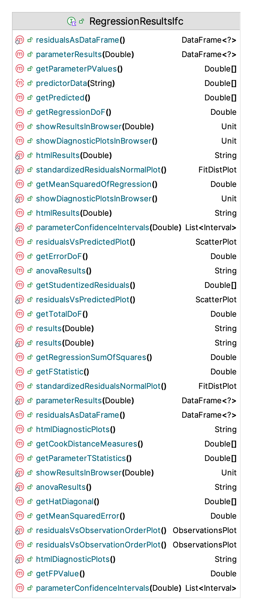
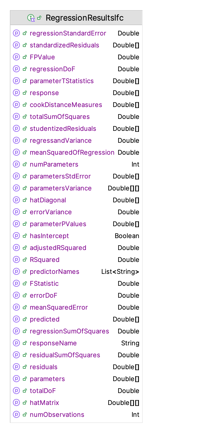
Figure 10.6: KSL Linear Regression Support
The functionality includes support for performing the ANOVA analysis, estimating the parameters, displaying diagnostic plots, and for performing an analysis of the residuals. The most useful functionality is to use the showResultsInBrowser() and showDiagnosticPlotsInBrowser() functions.
The performing of an regression analysis is made possible by the RegressionData class as shown in Figure 10.7. The key purpose of this class is to organize the regression matrix and the response array for analysis. The predictor names and response names are also specified.
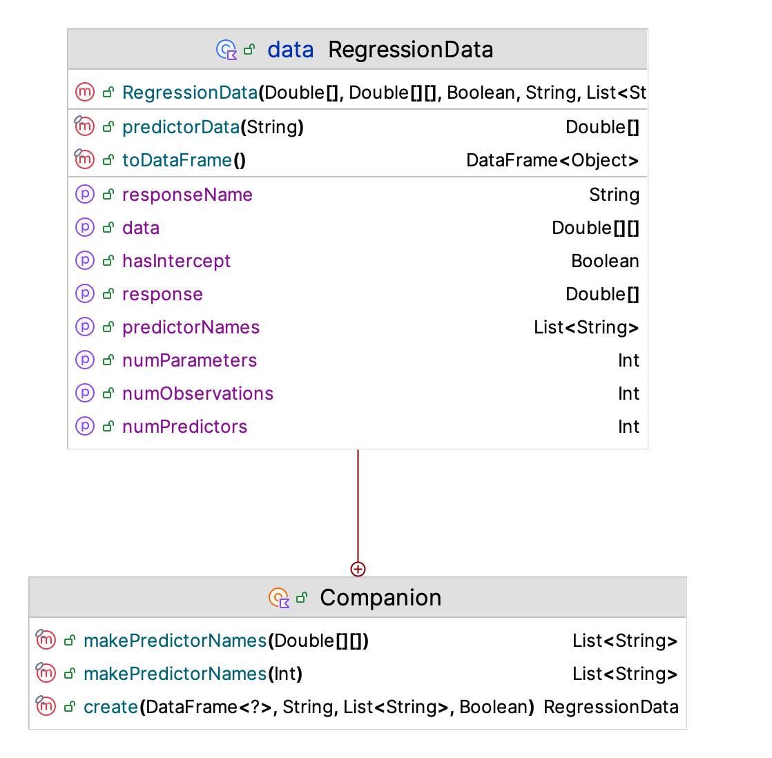
Figure 10.7: KSL Regression Data
The OLSRegression class with the following signature performs the regression. Notice that there is a constructor that will use a data frame, which requires the specification of the column name of the response variable and the columns needed for the predictor (regressor) variables.
class OLSRegression(regressionData: RegressionData) : RegressionResultsIfc {

    /**
     *  Create the regression data from a data frame. The data frame
     *  must have a column with the response name [responseName] and
     *  columns with the names in the list [predictorNames]. The
     *  data type of these columns must be Double. [hasIntercept] indicates
     *  if the regression should include an intercept term. The default is
     *  true. The data in the data frame does not need to have a column
     *  for estimating the intercept.
     */
    constructor(
        df: AnyFrame,
        responseName: String,
        predictorNames: List<String>,
        hasIntercept: Boolean = true
    ) : this(RegressionData.create(df, responseName, predictorNames, hasIntercept))
The KSL regression functionality is available with in the ksl.utilities.statistics package.