2.3 How the Discrete-Event Clock Works
This section introduces the concept of how time evolves in a discrete event simulation. This topic will also be revisited in future chapters after you have developed a deeper understanding for many of the underlying elements of simulation modeling.
In discrete-event dynamic systems, an event is something that happens at an instant in time which corresponds to a change in system state. An event can be conceptualized as a transmission of information that causes an action resulting in a change in system state. Let’s consider a simple bank which has two tellers that serve customers from a single waiting line. In this situation, the system of interest is the bank tellers (whether they are idle or busy) and any customers waiting in the line. Assume that the bank opens at 9 am, which can be used to designate time zero for the simulation. It should be clear that if the bank does not have any customers arrive during the day that the state of the bank will not change. In addition, when a customer arrives, the number of customers in the bank will increase by one. In other words, an arrival of a customer will change the state of the bank. Thus, the arrival of a customer can be considered an event.
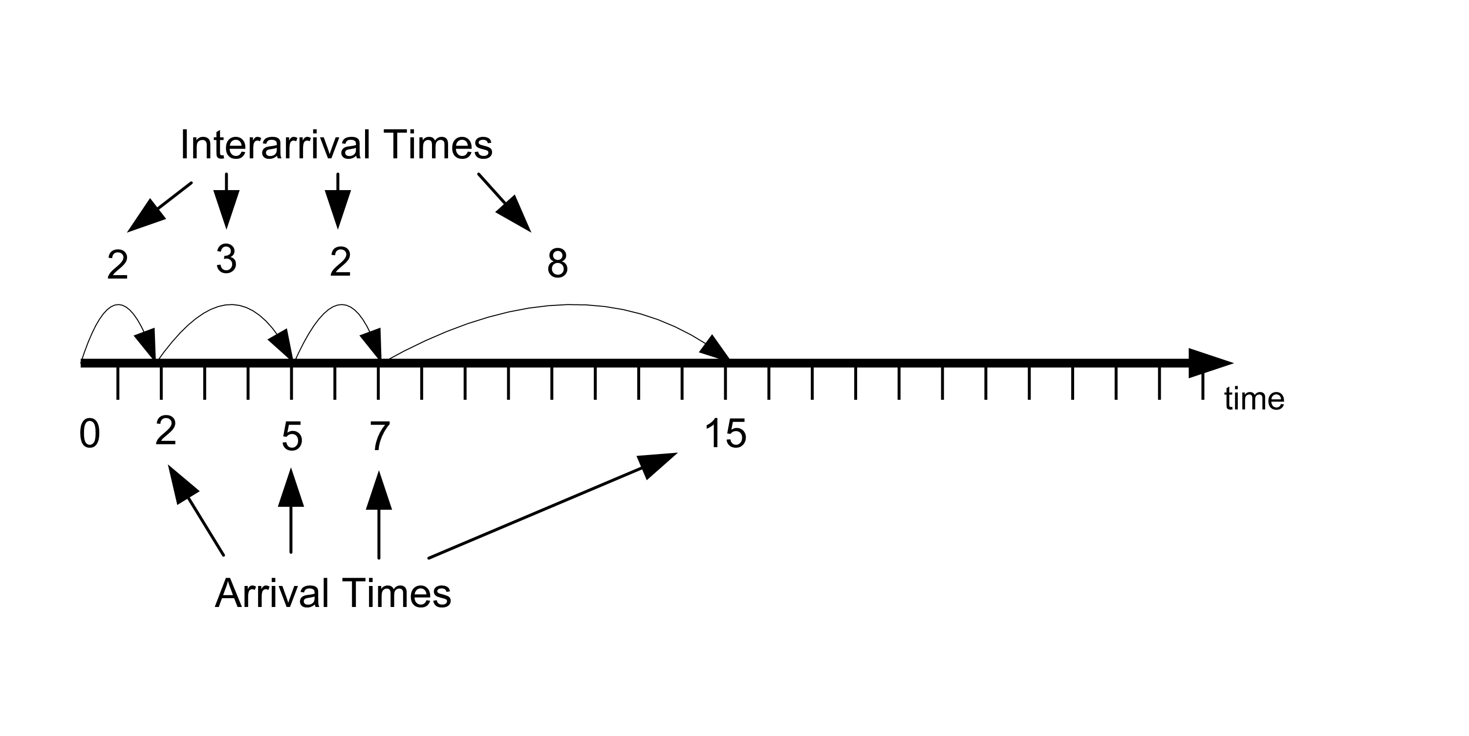
Figure 2.14: Customer arrival process
| Customer | Time of arrival | Time between arrival |
|---|---|---|
| 1 | 2 | 2 |
| 2 | 5 | 3 |
| 3 | 7 | 2 |
| 4 | 15 | 8 |
Figure 2.14 illustrates a time line of customer arrival events. The values for the arrival times in Table 2.2 have been rounded to whole numbers, but in general the arrival times can be any real valued numbers greater than zero. According to the figure, the first customer arrives at time two and there is an elapse of three minutes before customer 2 arrives at time five. From the discrete-event perspective, nothing is happening in the bank from time \([0,2)\); however, at time 2, an arrival event occurs and the subsequent actions associated with this event need to be accounted for with respect to the state of the system. An event denotes an instance of time that changes the state of the system. Since an event causes actions that result in a change of system state, it is natural to ask: What are the actions that occur when a customer arrives to the bank?
The customer enters the waiting line.
If there is an available teller, the customer will immediately exit the line and the available teller will begin to provide service.
If there are no tellers available, the customer will remain waiting in the line until a teller becomes available.
Now, consider the arrival of the first customer. Since the bank opens at 9 am with no customer and all the tellers idle, the first customer will enter and immediately exit the queue at time 9:02 am (or time 2) and then begin service. After the customer completes service, the customer will exit the bank. When a customer completes service (and departs the bank) the number of customers in the bank will decrease by one. It should be clear that some actions need to occur when a customer completes service. These actions correspond to the second event associated with this system: the customer service completion event. What are the actions that occur at this event?
The customer departs the bank.
If there are waiting customers, the teller indicates to the next customer that he/she will serve the customer. The customer will exit the waiting line and will begin service with the teller.
If there are no waiting customers, then the teller will become idle.
Figure 2.15 contains the service times for each of the four customers that arrived in Figure 2.14. Examine the figure with respect to customer 1. Based on the figure, customer 1 can enter service at time two because there were no other customers present in the bank. Suppose that it is now 9:02 am (time 2) and that the service time of customer 1 is known in advance to be 8 minutes as indicated in Table 2.3. From this information, the time that customer 1 is going to complete service can be pre-computed. From the information in the figure, customer 1 will complete service at time 10 (current time + service time = 2 + 8 = 10). Thus, it should be apparent, that for you to recreate the bank’s behavior over a time period that you must have knowledge of the customer’s service times. The service time of each customer coupled with the knowledge of when the customer began service allows the time that the customer will complete service and depart the bank to be computed in advance. A careful inspection of Figure 2.15 and knowledge of how banks operate should indicate that a customer will begin service either immediately upon arrival (when a teller is available) or coinciding with when another customer departs the bank after being served. This latter situation occurs when the queue is not empty after a customer completes service. The times that service completions occur and the times that arrivals occur constitute the pertinent events for simulating this banking system.
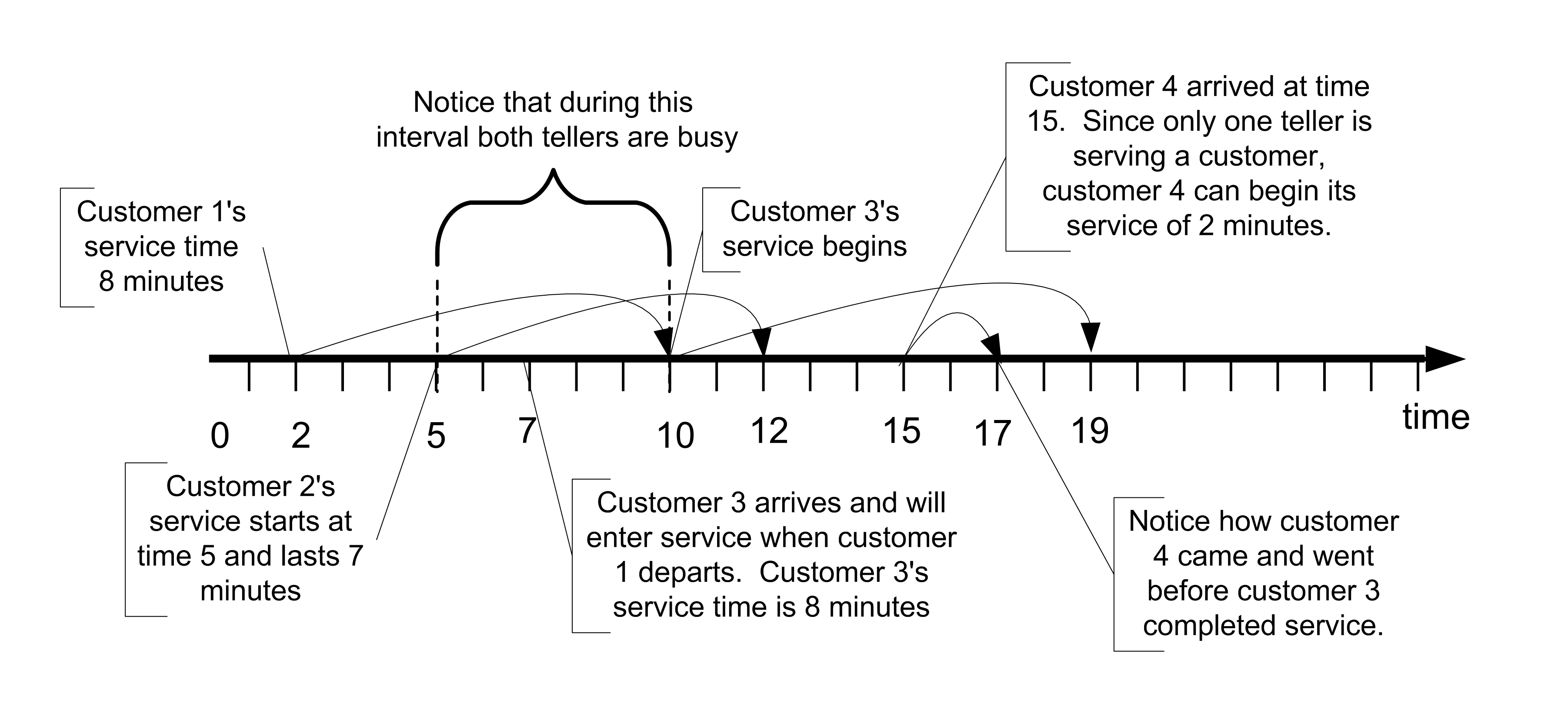
Figure 2.15: Customer service process
| Customer | Service Time Started | Service Time | Service Time Completed |
|---|---|---|---|
| 1 | 2 | 8 | 10 |
| 2 | 5 | 7 | 12 |
| 3 | 10 | 9 | 19 |
| 4 | 15 | 2 | 17 |
If the arrival and the service completion events are combined, then the time ordered sequence of events for the system can be determined. Figure 2.16 illustrates the events ordered by time from smallest event time to largest event time. Suppose you are standing at time two. Looking forward, the next event to occur will be at time 5 when the second customer arrives. When you simulate a system, you must be able to generate a sequence of events so that, at the occurrence of each event, the appropriate actions are invoked that change the state of the system.
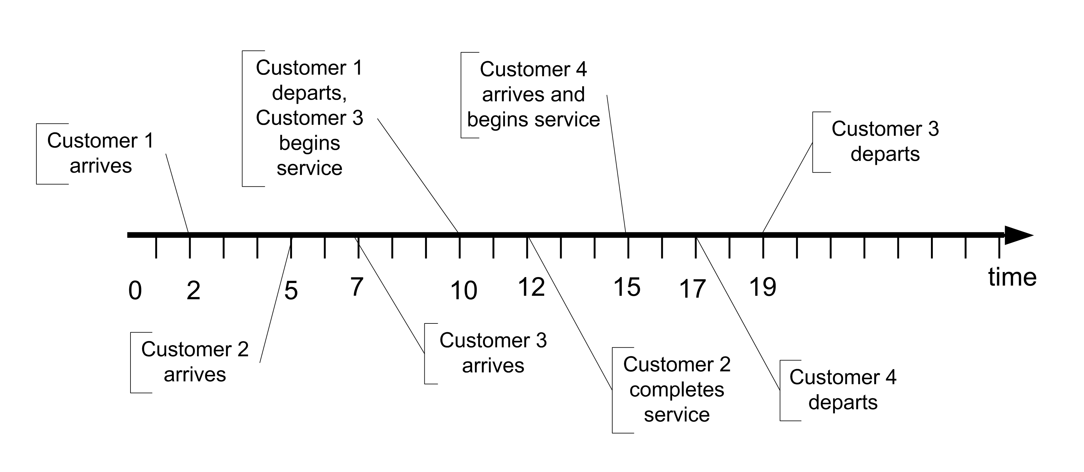
Figure 2.16: Events ordered by time
In the following table, \(c_i\) represents the \(i^{th}\) customer and \(s_j\) represents the \(j^{th}\) teller.
| Time | Event | Comment |
|---|---|---|
| 0 | Bank 0pens | |
| 2 | Arrival | \(c_1\) arrives, enters service for 8 min., \(s_1\) becomes busy |
| 5 | Arrival | \(c_2\) arrives, enters service for 7 min., the \(s_2\) becomes busy |
| 7 | Arrival | \(c_3\) arrives, waits in queue |
| 10 | Service Completion | \(c_1\) completes service, \(c_3\) exits queue, enters service for 9 min. |
| 12 | Service Completion | \(c_2\) completes service, queue is empty, \(s_2\) becomes idle |
| 15 | Arrival | \(c_4\) arrives, enters service for 2 min., \(s_2\) becomes busy |
| 17 | Service Completion | \(c_4\) completes service, \(s_2\) becomes idle |
| 19 | Service Completion | \(c_3\) completes service, \(s_1\) becomes idle |
The real system will simply evolve over time; however, a simulation of the system must recreate the events. In simulation, events are created by adding additional logic to the normal state changing actions. This additional logic is responsible for scheduling future events that are implied by the actions of the current event. For example, when a customer arrives, the time to the next arrival can be generated and scheduled to occur at some future time. This can be done by generating the time until the next arrival and adding it to the current time to determine the actual arrival time. Thus, all the arrival times do not need to be pre-computed prior to the start of the simulation. For example, at time two, customer 1 arrived. Customer 2 arrives at time 5. Thus, the time between arrivals (3 minutes) is added to the current time and customer 2’s arrival at time 5 is scheduled to occur. Every time an arrival occurs this additional logic is invoked to ensure that more arrivals will continue within the simulation.
Adding additional scheduling logic also occurs for service completion events. For example, since customer 1 immediately enters service at time 2, the service completion of customer 1 can be scheduled to occur at time 12 (current time + service time = 2 + 10 = 12). Notice that other events may have already been scheduled for times less than time 12. In addition, other events may be inserted before the service completion at time 12 actually occurs. From this, you should begin to get a feeling for how a computer program can implement some of these ideas.
Based on this intuitive notion for how a computer simulation may execute, you should realize that computer logic processing need only occur at the event times. That is, the state of the system does not change between events. Thus, it is not necessary to step incrementally through time checking to see if something happens at time 0.1, 0.2, 0.3, etc. (or whatever time scale you envision that is fine enough to not miss any events). Thus, in a discrete-event dynamic system simulation the clock does not “tick” at regular intervals. Instead, the simulation clock jumps from event time to event time. As the simulation moves from the current event to the next event, the current simulation time is updated to the time of the next event and any changes to the system associated with the next event are executed. This allows the simulation to evolve over time.