6.8 Exercises
Exercise 6.1 As part of a diabetes prevention program, a clinic is considering setting up a screening service in a local mall. They are considering two designs: Design A: After waiting in a single line, each walk-in patient is served by one of three available nurses. Each nurse has their own booth, where the patient is first asked some medical health questions, then the patient’s blood pressure and vitals are taken, finally, a glucose test is performed to check for diabetes. In this design, each nurse performs the tasks in sequence for the patient. If the glucose test indicates a chance of diabetes, the patient is sent to a separate clerk to schedule a follow-up at the clinic. If the test is not positive, then the patient departs.
Design B: After waiting in a single line, each walk-in is served in order by a clerk who takes the patient’s health information, a nurse who takes the patient’s blood pressure and vitals, and another nurse who performs the diabetes test. If the glucose test indicates a chance of diabetes, the patient is sent to a separate clerk to schedule a follow-up at the clinic. If the test is not positive, then the patient departs. In this configuration, there is no room for the patient to wait between the tasks; therefore, a patient who as had their health information taken cannot move ahead unless the nurse taking the vital signs is available. Also, a patient having their glucose tested must leave that station before the patient in blood pressure and vital checking can move ahead.
Patients arrive to the clinic according to non-stationary Poisson process. Assume that there is a 5% chance (stream 2) that the glucose test will be positive. For design A, the time that it takes to have the paperwork completed, the vitals taken, and the glucose tested are all log-normally distributed with means of 6.5, 6.0, and 5.5 minutes respectively (streams 3, 4, 5). They all have a standard deviation of approximately 0.5 minutes. For design B, because of the specialization of the tasks, it is expected that the mean of the task times will decrease by 10%.
Assume that the mall opens at 10 am and that the system operates until 8 pm. During the time from 10 am to 12 noon the arrivals are less than the overall arrival rate. From 10 am to noon, the rate is only 6.5 per hour. From noon to 2 pm, the rate increases to 12.5 per hour. From 2 pm to 4 pm the traffic lightens up again, back to 6.5 per hour. From 4 pm to 6 pm, the rate is 12.5 per hour and finally from 6 pm to 8 pm, the rate is 9.5 per hour. Assume that the clinic is open from 10 am to 8 pm (10 hours each day) and that any patients in the clinic before 8 pm are still served. The distribution used to model the time that it takes to schedule a follow up visit is a WEIB(2.6, 7.3) distribution (use stream 6).
Make a statistically valid recommendation as to the best design based on the average system time of the patients. We want to be 95% confident of our recommendation to within 2 minutes.Exercise 6.3 Suppose a service facility consists of two stations in series (tandem), each with its own FIFO queue. Each station consists of a queue and a single server. A customer completing service at station 1 proceeds to station 2, while a customer completing service at station 2 leaves the facility. Assume that the inter-arrival times of customers to station 1 are IID exponential random variables with a mean of 1.25 minutes. Service times of customers at station 1 are exponential random variables with a mean of 0.7 minute, and at station 2 are exponential random variables with mean 0.9 minute.
Suppose that there is limited space at the second station. In particular, there is room for 1 customer to be in service at the second station and room for only 1 customer to wait at the second station. A customer completing service at the first station will not leave the service area at the first station unless there is a space available for it to wait at the second station. In other words, the customer will not release the server at the first station unless it can move to the second station.
Develop a model for this system using the STATION and ROUTE modules. Run the simulation for exactly 20000 minutes with a warm up period of 2000 minutes for 20 replications and estimate for each station the expected average delay in queue for the customer, the expected time-average number of customers in queue, and the expected utilization. In addition, estimate the average number of customers in the system and the average time spent in the system.Use a resource to model the waiting space at the second station. Ensure that a customer leaving the first station does not release its resource until it is able to seize the space at the second station.
Use a HOLD module with the wait and signal option to model this situation. Compare your results to those obtained in part (a).
Use a HOLD module with the scan for condition option to model this situation. Compare your results to parts (a) and (b).
Suppose now there is a travel time from the exit of station 1 to the arrival to station 2. Assume that this travel time is distributed uniformly between 0 and 2 minutes. Modify your simulation for part (a) and rerun it under the same conditions as in part (a).
Using simulate the performance of this system using \(Q = 4\) and \(r =3\). Report the average inventory on hand, the cost for operating the policy, the average number of back-orders, and the probability of a stock out for your model.
Now suppose that the lead-time is stochastic and governed by a lognormal distribution with a mean of 45 days and a standard deviation of 7 days. What assumptions do you have to make to simulate this situation? Simulate this situation and compare/contrast the results with part (a).
Verify your results for part (a) using results from analytical inventory theory.
Exercise 6.6 The Super Ready Auto Club has been serving customers for many years. The Super Ready Auto Club provides club, travel, and financial services to its members. One of its most popular services includes auto touring and emergency road service. Travel provides cruise packages, airline travel, and other vacation packages with special discounts for members. Finally, the financial services issues credit cards for members at special interest rates.
Super Ready Auto Club has regional call centers that handle incoming calls from members within a given region of the country. Table 6.6 presents the mean of the number of calls, recorded on an hourly basis over a period of 7 days, aggregated over a three state region.
The three types of service calls occur with 60% for auto service, 35% for credit card services, and 15% for travel services during the 8 am to 8 pm time frame. For the other hours of the day, the proportion changes to 90% for auto service, 10% for credit card services, and 0% for travel services. A sample of call service times were recorded for each of the types as shown in Tables 6.6, 6.7, (6.8, and (6.8. You can find this data in the chapter files that accompany this chapter in the spreasheet called Super Ready Auto Club.xlsx.
Call center operators cost $18 per hour including fringe benefits. It is important that the probability of a call waiting more than 3 minutes for an operator be less than 10%. Find a minimum cost staffing plan for each hour of the day for each day of the week that on-average meets the call probability waiting criteria. Measure the waiting time for a call, the average number of calls waiting, and the utilization of the operators. In addition, measure the waiting time of the calls by type. The data for this exercise is available within the files associated with this chapter.
What happens to the waiting times if road-side assistance calls are given priority over the credit card and travel service calls?
Consider how you would handle the following work rules. The operators should get a 10 minute break every 2 hours and a 30 minute food/beverage break every 4 hours. Discuss how you would staff the center under these conditions ensuring that there is always someone present (i.e. they are not all on break at the same time).
| Hour | Mon | Tue | Wed | Thur | Fri | Sat | Sun |
|---|---|---|---|---|---|---|---|
| 1 | 6.7 | 6.1 | 8.7 | 8.9 | 5.6 | 6.2 | 9.4 |
| 2 | 9.7 | 9.4 | 9.3 | 7.1 | 1.4 | 7.0 | 8.8 |
| 3 | 8.5 | 6.0 | 70.4 | 8.6 | 7.9 | 7.8 | 13.4 |
| 4 | 9.0 | 10.0 | 6.8 | 8.3 | 6.4 | 6.3 | 6.7 |
| 5 | 6.8 | 9.2 | 10.9 | 44.9 | 8.2 | 6.5 | 7.5 |
| 6 | 8.5 | 4.2 | 1.4 | 6.3 | 7.5 | 7.8 | 8.0 |
| 7 | 6.7 | 6.9 | 9.0 | 8.9 | 6.7 | 46.2 | 9.8 |
| 8 | 38.2 | 35.0 | 75.8 | 57.8 | 37.2 | 82.5 | 78.8 |
| 9 | 20.0 | 77.6 | 48.7 | 25.9 | 67.1 | 28.1 | 99.2 |
| 10 | 76.2 | 75.4 | 71.1 | 51.3 | 86.2 | 106.9 | 42.0 |
| 11 | 92.5 | 105.4 | 28.2 | 100.2 | 90.9 | 92.4 | 43.6 |
| 12 | 76.4 | 37.3 | 37.3 | 77.8 | 60.3 | 37.9 | 68.9 |
| 13 | 79.1 | 64.2 | 25.4 | 76.8 | 65.1 | 77.9 | 116.6 |
| 14 | 75.2 | 102.2 | 64.1 | 48.7 | 93.3 | 64.5 | 39.5 |
| 15 | 117.9 | 26.8 | 43.8 | 80.1 | 86.4 | 96.8 | 52.1 |
| 16 | 100.2 | 85.9 | 54.3 | 144.7 | 70.9 | 167.9 | 153.5 |
| 17 | 52.7 | 64.7 | 94.7 | 94.6 | 152.2 | 98.0 | 63.7 |
| 18 | 65.3 | 114.9 | 124.9 | 213.9 | 91.5 | 135.7 | 79.8 |
| 19 | 126.1 | 69.6 | 89.4 | 43.7 | 62.7 | 111.9 | 180.5 |
| 20 | 116.6 | 70.2 | 116.8 | 99.6 | 113.0 | 84.3 | 64.1 |
| 21 | 38.6 | 20.5 | 7.6 | 3.8 | 58.6 | 50.8 | 68.5 |
| 22 | 8.5 | 17.1 | 8.8 | 13.5 | 8.2 | 68.1 | 7.8 |
| 23 | 9.8 | 48.9 | 8.9 | 95.4 | 40.8 | 58.5 | 44.1 |
| 24 | 9.6 | 1.3 | 28.5 | 9.6 | 32.2 | 74.5 | 46.7 |
| 33.6 | 34.0 | 33.2 | 31.3 | 32.3 | 32.1 | 39.0 | 35.2 | 37.6 | 37.4 |
| 32.3 | 37.2 | 39.3 | 32.1 | 34.7 | 35.1 | 33.6 | 32.8 | 32.8 | 40.0 |
| 37.8 | 38.0 | 42.4 | 37.4 | 36.6 | 36.6 | 33.3 | 34.7 | 30.2 | 33.1 |
| 36.8 | 34.4 | 36.4 | 35.9 | 32.6 | 37.6 | 36.7 | 32.3 | 40.0 | 37.0 |
| 36.0 | 34.6 | 33.9 | 31.7 | 33.8 | 39.3 | 37.8 | 33.7 | 35.2 | 38.2 |
| 34.6 | 33.5 | 36.3 | 38.9 | 35.5 | 35.2 | 35.0 | 33.8 | 35.8 | 35.8 |
| 38.2 | 38.8 | 35.7 | 38.7 | 30.0 | 33.6 | 33.4 | 34.7 | 35.1 | 35.5 |
| 34.0 | 33.2 | 33.7 | 32.5 | 28.9 | 34.4 | 34.2 | 31.4 | 38.7 | 35.3 |
| 35.5 | 39.4 | 32.6 | 36.2 | 33.2 | 39.3 | 41.1 | 34.3 | 38.6 | 33.0 |
| 35.3 | 38.1 | 33.5 | 34.0 | 36.4 | 33.6 | 43.1 | 37.2 | 35.6 | 36.0 |
| 52.2 | 23.7 | 33.9 | 30.5 | 18.2 | 45.2 | 38.4 | 49.8 | 53.9 | 38.8 |
| 33.4 | 44.2 | 28.4 | 49.0 | 24.9 | 46.4 | 35.8 | 40.3 | 16.3 | 41.4 |
| 63.1 | 37.5 | 33.5 | 48.0 | 27.6 | 38.2 | 28.6 | 35.2 | 24.5 | 42.9 |
| 38.9 | 19.8 | 32.7 | 41.4 | 42.7 | 27.4 | 38.7 | 30.1 | 39.6 | 53.5 |
| 28.8 | 42.2 | 42.4 | 29.2 | 22.7 | 50.9 | 34.2 | 53.1 | 18.5 | 26.5 |
| 40.9 | 20.7 | 36.6 | 33.7 | 26.4 | 32.8 | 25.1 | 39.7 | 30.9 | 34.2 |
| 35.5 | 31.8 | 27.2 | 28.6 | 26.9 | 30.6 | 26.1 | 23.2 | 33.3 | 35.0 |
| 29.6 | 31.6 | 29.9 | 28.5 | 29.3 | 30.6 | 31.2 | 26.7 | 25.7 | 41.2 |
| 27.5 | 52.0 | 27.3 | 69.0 | 34.2 | 31.4 | 21.9 | 29.8 | 31.4 | 46.1 |
| 23.8 | 35.9 | 41.5 | 51.0 | 17.9 | 33.9 | 32.2 | 26.5 | 25.0 | 54.6 |
| 13.5 | 10.1 | 14.4 | 13.9 | 14.2 | 11.4 | 11.0 | 14.4 | 12.0 | 14.4 |
| 14.4 | 13.5 | 13.4 | 14.5 | 14.8 | 14.9 | 13.2 | 11.0 | 14.9 | 15.0 |
| 14.7 | 14.3 | 12.3 | 14.8 | 12.4 | 14.9 | 15.0 | 14.0 | 14.6 | 14.6 |
| 15.0 | 10.3 | 11.3 | 15.0 | 15.0 | 15.0 | 14.9 | 14.8 | 11.5 | 11.9 |
| 13.5 | 14.9 | 11.0 | 10.8 | 15.0 | 13.8 | 13.8 | 14.5 | 14.3 | 14.0 |
| 14.9 | 10.9 | 13.9 | 13.5 | 15.0 | 14.4 | 13.2 | 15.0 | 14.5 | 14.4 |
| 15.0 | 14.5 | 14.5 | 14.9 | 11.6 | 13.6 | 12.4 | 11.9 | 11.6 | 15.0 |
| 11.1 | 13.7 | 13.9 | 14.6 | 11.5 | 14.4 | 15.0 | 10.7 | 10.4 | 14.5 |
| 12.3 | 13.8 | 14.7 | 13.8 | 14.7 | 14.8 | 14.9 | 14.2 | 12.9 | 14.3 |
| 14.5 | 11.5 | 12.1 | 14.3 | 13.6 | 14.1 | 12.6 | 11.7 | 14.7 | 13.4 |
Exercise 6.7 The test and repair system described in Chapter 4 has 3 testing stations, a diagnostic station, and a repair station. Suppose that the machines at the test station are subject to random failures. The time between failures is distributed according to an exponential distribution with a mean of 240 minutes and is based on busy time. Whenever, a test station fails, the testing software must be reloaded, which takes between 10 and 15 minutes uniformly distributed. The diagnostic machine is also subject to usage failures. The number of uses to failure is distributed according to a geometric distribution with a mean of 100. The time to repair the diagnostic machine is uniformly distributed in the range of 15 to 25 minutes. Examine the effect of explicitly modeling the machine failures for this system in terms of risks associated with meeting the terms of the contract.
Exercise 6.8 A proposal for a remodeled Sly’s Convenience Store has 6 gas pumps each having their own waiting line. The inter-arrival time distribution of the arriving cars is Poisson with a mean of 1.25 per minute. The time to fill up and pay for the purchase is exponentially distributed with a mean of 6 minutes. Arriving customers choose the pump that has the least number of cars (waiting or using the pump). Each pump has room to handle 3 cars (1 in service and 2 waiting). Cars that cannot get a pump wait in an overall line to enter a line for a pump. The long run performance of the system is of interest.
Estimate the average time in the system for a customer, the average number of customers waiting in each line, the overall line, and in the system, and estimate the percentage of time that there are 1, 2, 3 customers waiting in each line. In addition, the percentage of time that there are 1, 2, 3, 4 or more customers waiting to enter a pump line should be estimated. Assume that each car is between 16 and 18 feet in length. About how much space in the overall line would you recommend for the convenience store.
Occasionally, a pump will fail. The time between pump failures is distributed according to an exponential distribution with a mean of 40 hours and is based on clock time (not busy time). The time to service a pump is exponentially distributed with a mean of 4 hours. For simplicity assume that when a pump fails the customer using the pump is able to complete service before the pump is unusable and ignore the fact that some customers may be in line when the pump fails. Simulate the system under these new conditions and estimate the same quantities as requested in part (a). In addition, estimate the percentage of time that each pump spends idle, busy, or failed. Make sure that newly arriving customers do not decide to enter the line of a pump that has failed.
The assumption that a person waiting in line when a pump fails stays in line is unrealistic. Still assume that a customer receiving service when the pump fails can complete service, but now allow waiting customers to exit their line and rejoin the overall line if a pump fails while they are in line. Compare the results of this new model with those of part (b).
Exercise 6.9 Apply the concepts of generic station modeling to the system described in Exercise 5.18. Be sure to show that your results are essentially the same with and without generic modeling.
Exercise 6.10 Suppose the shuttle bus system described in Section 6.6.3 now has 3 bus stops. Passengers arrive to bus stop 1 according to a Poisson arrival process with a mean rate of 6 per hour. Passengers arrive to bus stop 2 according to a Poisson arrival process with a mean rate of 10 per hour. Passengers arrive to bus stop 3 according to a Poisson arrival process with a mean rate of 12 per hour. Thirty percent of customers arrive to stop 1 desire to go to stop 2 with the remaining going to stop 3. For those passengers arriving to stop 2, 75% want to go to stop 1 and 25% want to go to stop 3. Finally, for those passengers that originate at stop 3, 40% want to go to stop 1 and 60% want to go to stop 2. The shuttle bus now has 20 seats. The loading and unloading times per passenger are still the same as in the example and the travel time between stops is still the same. Simulate this system for 8 hours of operation and estimate the average waiting time of the passengers, the average system time of the passengers, and the average number of passengers left at the stop because the bus was full.
Exercise 6.11 Reconsider the STEM Career Fair Mixer Example 6.1. The results indicated that the utilization of the JHBunt recruiters was still high, around 90%, and the MalWart recruiters was low, around 50% after making the resource schedule changes. Design a schedule that gets both recruiting stations to about 80% during the peak period.
Exercise 6.12 This problem examines a single item, multi-stage, serial production system using a kanban control system. The word kanban is Japanese for card. A kanban is simply a card that authorizes production. Kanban based control systems are designed to limit the amount of inventory in production. While there are many variations of kanban control, this problem considers a simplified system with the following characteristics.
A series of work centers
Each work center consists of one or more identical machines with an input queue feeding the machines that is essentially infinite.
Each work center also has an output queue where completed parts are held to await being sent to the next work center.
Each work center has a schedule board where requests for new parts are posted
Customer orders arrive randomly at the last work center to request parts. If there are no parts available then the customers will wait in a queue until a finished part is placed in the output buffer of the last work center.
Figure 6.89 illustrates a production flow line consisting of kanban based work centers.
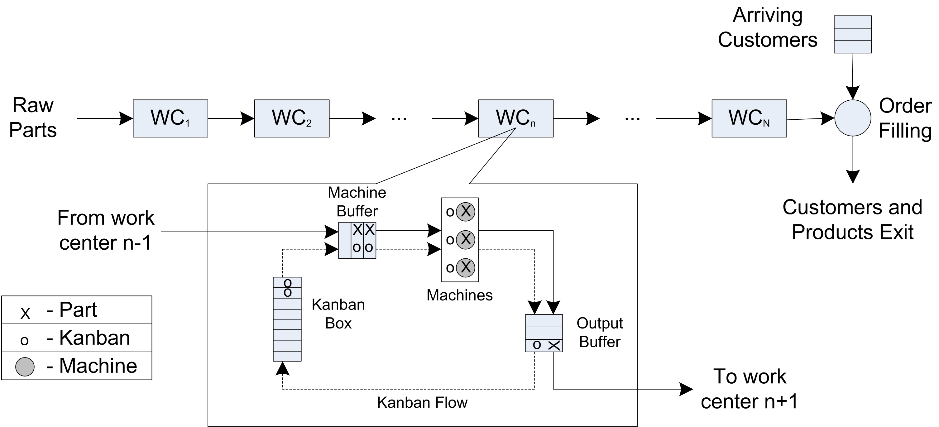
Figure 6.89: Kanban workcenter
Raw parts enter at the first work center and proceed, as needed, through each work center until eventually being completed as finished parts at the last work center. Finished parts are used to satisfy end customer demand.
A detailed view of an individual kanban based work center is also shown in the figure. Here parts from the previous work center are matched with an available kanban to proceed through the machining center. Parts completed by the machining center are placed in the output buffer (along with their kanban) to await demand from the next work center.
An individual work center works as follows:
Each work center has a finite number of kanbans, \(K_n \geq 1\)
Every part must acquire one of these kanbans in order to enter a given work center and begin processing at the machining center. The part holds the kanban throughout it stay in the work center (including the time it is in the output buffer).
Unattached kanbans are stored on the schedule board and are considered as requests for additional parts from the previous work center.
When a part completes processing at the machines, the system checks to see if there is a free kanban at the next work center. If there is a free kanban at the next work center, the part releases its current kanban and seizes the available kanban from the next work center. The part then proceeds to the next work center to begin processing at the machines. If a kanban is not available at the next work center, the part is place in the output buffer of the work center to await a signal that there is a free kanban available at the next station.
Whenever a kanban is released at the work center it signals any waiting parts in the output buffer of its feeder work center. If there is a waiting part in the output buffer when the signal occurs, the part leaves the output buffer, releasing it current kanban, and seizing the kanban of the next station. It then proceeds to the next work center to be processed by the machines.
For the first work center in the line, whenever it needs a part (i.e. when one of its kanbans are released) a new part is created and immediately enters the work center. For the last work center, a kanban in its output buffer is not released until a customer arrives and takes away the finished part to which the kanban was attached. Consider a three work center system. Let \(K_N\) be the number of Kanbans and let \(c_n\) be the number of machines at work center \(n, n = 1,2,3\). Let’s assume that each machine’s service time distribution is an exponential distribution with service rate \(\mu_n\). Demands from customers arrive to the system according to a Poisson process with rate \(\lambda\). As an added twist assume that the queue of arriving customers can be limited. In other words, the customer queue has a finite waiting capacity, say \(C_q\). If a customer arrives when there are \(C_q\) customers already in the customer queue they do not enter the system. Build a simulation model to simulate the following case:
| \(c_1\) | \(c_2\) | \(c_3\) |
|---|---|---|
| 1 | 1 | 1 |
| \(k_1\) | \(k_2\) | \(k_3\) |
| 2 | 2 | 2 |
| \(\mu_1\) | \(\mu_2\) | \(\mu_3\) |
| 3 | 3 | 3 |
where \(\lambda = 2\) and \(C_q = \infty\) with all rates per hour. Estimate the average hourly throughput for the production line. That is, the number of items produced per hour. Run the simulation for 10 replications of length 15000 hours with a warm up period of 5000 hours. Suppose \(C_q = 5\), what is the effect on the system.