5.1 A Spreadsheet Example
To illustrate the challenges related to infinite horizon simulations, a simple spreadsheet simulation was developed for a M/M/1 queue as introduced in Chapter 2. The spreadsheet model is provided in the spreadsheet file MM1-QueueingSimulation.xlsm that accompanies this chapter. The immediate feedback from a spreadsheet model should facilitate understanding the concepts. Consider a single server queuing system as illustrated Figure 5.1.
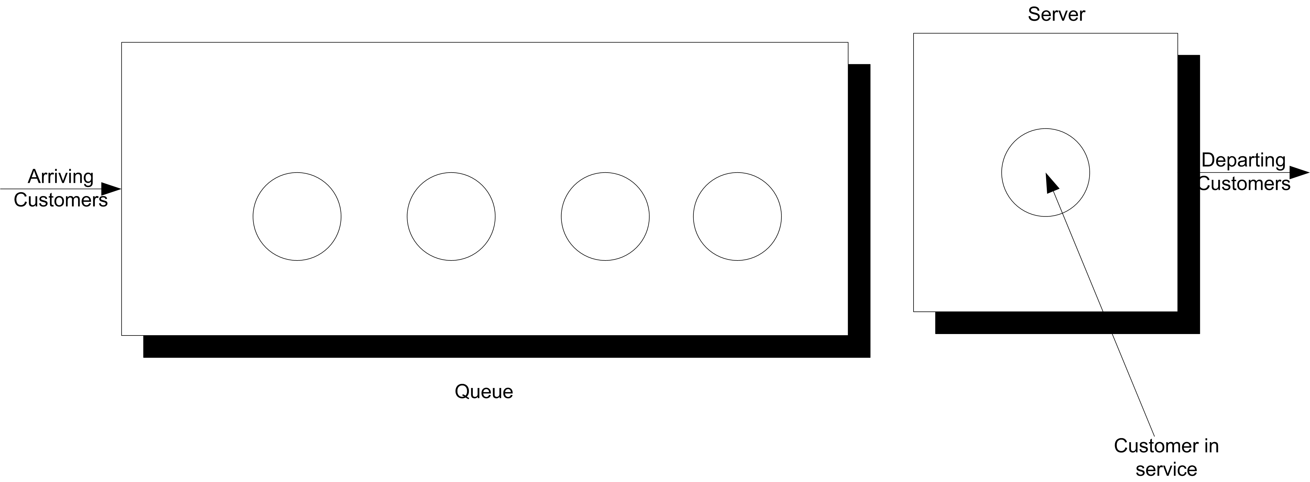
Figure 5.1: Single server queueing system
For a single server queueing system, there is an equation that allows the computation of the waiting times of each of the customers based on knowledge of the arrival and service times. Let \(X_1, X_2, \ldots\) represent the successive service times and \(Y_1, Y_2, \ldots\) represent the successive inter-arrival times for each of the customers that visit the queue. Let \(E[Y_i] = 1/\lambda\) be the mean of the inter-arrival times so that \(\lambda\) is the mean arrival rate. Let \(E[Y_i] = 1/\mu\) be the mean of the service times so that \(\mu\) is the mean service rate. Let \(W_i\) be the waiting time in the queue for the \(i^{th}\) customer. That is, the time between when the customer arrives until they enter service.
Lindley’s equation, see (Gross and Harris 1998), relates the waiting time to the arrivals and services as follows:
\[W_{i+1} = max(0, W_i + X_i - Y_i)\]
The relationship says that the time that the \((i + 1)^{st}\) customer must wait is the time the \(i^{th}\) waited, plus the \(i^{th}\) customer’s service time, \(X_i\) (because that customer is in front of the \(i^{th}\) customer), less the time between arrivals of the \(i^{th}\) and \((i + 1)^{st}\) customers, \(Y_i\). If \(W_i + X_i - Y_i\) is less than zero, then the (\((i + 1)^{st}\) customer arrived after the \(i^{th}\) finished service, and thus the waiting time for the \((i + 1)^{st}\) customer is zero, because his service starts immediately.
Suppose that \(X_i \sim exp(E[X_i] = 0.7)\) and \(Y_i \sim exp(E[Y_i] = 1.0)\). This is a M/M/1 queue with \(\lambda\) = 1 and \(\mu\) = 10/7. Thus, using the equations given in Chapter 2 or Appendix C, yields:
\[\rho = 0.7\]
\[L_q = \dfrac{0.7 \times 0.7}{1 - 0.7} = 1.6\bar{33}\]
\[W_q = \dfrac{L_q}{\lambda} = 1.6\bar{33} \; \text{minutes}\]
The spreadsheet model involves generating \(X_i\) and \(Y_i\) as well as implementing Lindley’s equation within the rows of the spreadsheet. Figure 5.2 shows some sample output from the simulation. The simulation was initialized with \(X_0\) = 0 and random draws for \(X_0\) and \(Y_0\). The generated values for \(X_i\) and \(Y_i\) are based on the inverse transform technique for exponential random variables with the cell formulas given in cells D24 and E24, as shown in Figure 5.3.
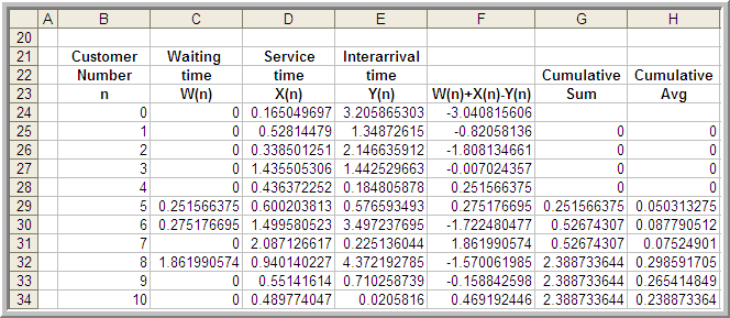
Figure 5.2: Spreadsheet for Lindley’s equation
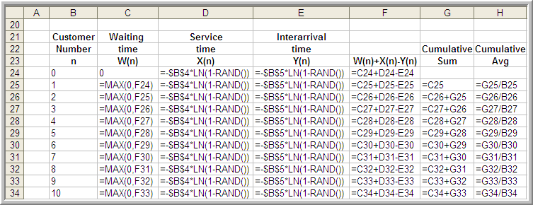
Figure 5.3: Spreadsheet formulas for queueing simulation
Figure 5.3 shows that cell F25 is based on the value of cell F24. This implements the recursive nature of Lindley’s formula. Column G holds the cumulative sum:
\[\sum_{i=1}^n W_i \; \text{for} \; n = 1,2,\ldots\]
and column H holds the cumulative average
\[\dfrac{1}{n} \sum_{i=1}^n W_i \; \text{for} \; n = 1,2,\ldots\]
Thus, cell H26 is the average of the first two customers, cell H27 is the average of the first 3 customers, and so forth. The final cell of column H represents the average of all the customer waiting times.
Figure 5.4 shows the results of the simulation across 1000 customers. The analytical results indicate that the true long-run expected waiting time in the queue is 1.633 minutes. The average over the 1000 customers in the simulation is 1.187 minutes. Figure 5.4 indicates that the sample average is significantly lower than the true expected average. Figure 5.5 presents the cumulative average plot of the first 1000 customers. As seen in the plot, the cumulative average starts out low and then eventually trends towards 1.2 minutes.
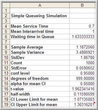
Figure 5.4: Results across 1000 customers
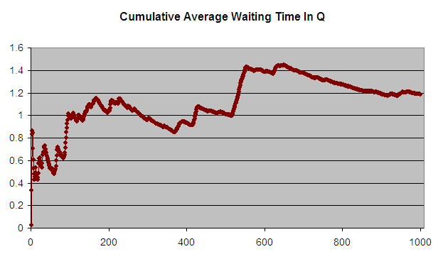
Figure 5.5: Cumulative average waiting time of 1000 customers
The first issue to consider with this data is independence. To do this you should analyze the 1000 observations in terms of its autocorrelation. From Figure 5.6, it is readily apparent that the data has strong positive correlation using the methods discussed in Appendix B. The lag-1 correlation for this data is estimated to be about 0.9. Figure 5.7 clearly indicates the strong first order linear dependence between \(W_i\) and \(W_{i-1}\). This positive dependence implies that if the previous customer waited a long time the next customer is likely to wait a long time. If the previous customer had a short wait, then the next customer is likely to have a short wait. This makes sense with respect to how a queue operates.
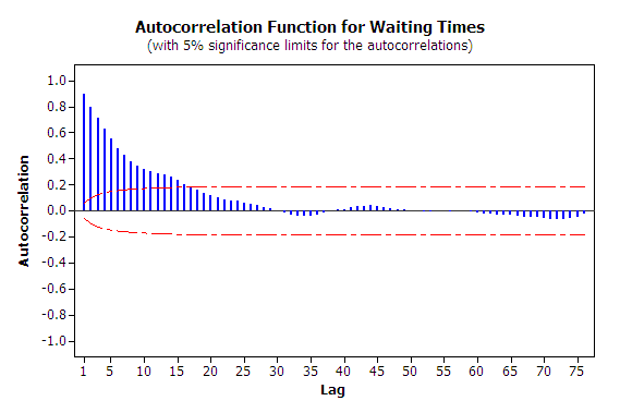
Figure 5.6: Autocorrelation plot for waiting times
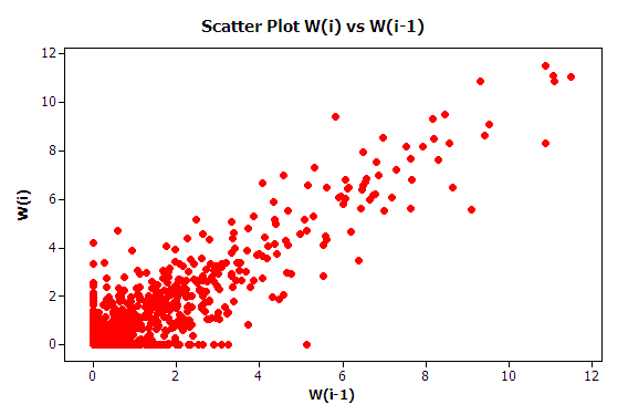
Figure 5.7: Lag 1 dependence for waiting times
Strong positive correlation has serious implications when developing confidence intervals on the mean customer waiting time because the usual estimator for the sample variance:
\[S^2(n) = \dfrac{1}{n - 1} \sum_{i=1}^n (X_i - \bar{X})^2\]
is a biased estimator for the true population variance when there is correlation in the observations. This issue will be re-examined when ways to mitigate these problems are discussed.
The second issue that needs to be discussed is that of the non-stationary behavior of the data. As discussed in Appendix B, non-stationary data indicates some dependence on time. More generally, non-stationary implies that the \(W_1, W_2,W_3, \ldots, W_n\) are not obtained from identical distributions.
Why should the distribution of \(W_1\) not be the same as the distribution of \(W_{1000}\)? The first customer is likely to enter the queue with no previous customers present and thus it is very likely that the first customer will experience little or no wait (the way \(W_0\) was initialize in this example allows a chance of waiting for the first customer). However, the \(1000^{th}\) customer may face an entirely different situation. Between the \(1^{st}\) and the \(1000^{th}\) customer there might likely be a line formed. In fact from the M/M/1 formula, it is known that the steady state expected number in the queue is 1.633. Clearly, the conditions that the \(1^{st}\) customer faces are different than those faced by the \(1000^{th}\) customer. Thus, the distributions of their waiting times are likely to be different.
Recall the definition of covariance stationary from Appendix B. A time series, \(W_1, W_2,W_3, \ldots, W_n\) is said to be covariance stationary if:
The mean exists and \(\theta = E[X_i]\), for i = 1,2,\(\ldots\), n
The variance exists and \(Var[X_i] = \sigma^2\) \(>\) 0, for i = 1,2,\(\ldots\), n
The lag-k autocorrelation, \(\rho_k = cor(X_i, X_{i+k})\), is not a function of i, i.e. the correlation between any two points in the series does not depend upon where the points are in the series, it depends only upon the distance between them in the series.
In the case of the customer waiting times, you should conclude from the discussion that it is very likely that \(\theta \neq E[X_i]\) and \(Var[X_i] \neq \sigma^2\) for each i = 1,2,\(\ldots\), n for the time series.
Do you think that is it likely that the distributions of \(W_{9999}\) and \(W_{10000}\) will be similar? The argument, that the \(9999^{th}\) customer is on average likely to experience similar conditions as the \(10000^{th}\) customer, sure seems reasonable. Figure 5.8 shows 10 different replications of the cumulative average for a 10000 customer simulation. This was developed using the sheet labeled 10000-Customers.
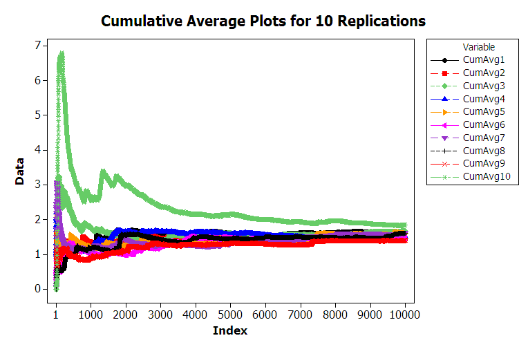
Figure 5.8: Multiple sample paths of queueing simulation
From the figure, you can see that the cumulative average plots can vary significantly over the 10000 customers with the average tracking above the true expected value, below the true expected value, and possibly towards the true expected value. Each of these plots was generated by pressing the F9 function key to have the spreadsheet recalculate with new random numbers and then capturing the observations onto another sheet for plotting. Essentially, this is like running a new replication. You are encouraged to try generating multiple sample paths using the provided spreadsheet. For the case of 10000 customers, you should notice that the cumulative average starts to approach the expected value of the steady state mean waiting time in the queue with increasing number of customers. This is the law of large numbers in action. It appears that it takes a period of time for the performance measure to warm up towards the true mean. Determining the warm up time will be the basic way to mitigate the problem of non-identical distributions.
From this discussion, you should conclude that the second basic statistical assumption of identically distributed data is not valid for within replication data. From this, you can also conclude that it is very likely that the data are not normally distributed. In fact, for the M/M/1 queue, it can be shown that the steady state distribution for the waiting time in the queue is not a normal distribution. Thus, all three of the basic statistical assumptions are violated for the within replication observations generated for this example. The problems associated with observations from within a replication need to be addressed in order to properly analyze infinite horizon simulation experiments.