8.5 Simulation Horizon and Run Parameters
The setting of the simulation horizon and the run parameters is challenging within this problem because of lack of guidance on this point from the problem description. Without specific guidance you will have to infer from the problem description how to proceed.
It can be inferred from the problem description that SMTesting is interested in using the new design over a period of time, which may be many months or years. In addition, the problem states that SMTesting wants all cost estimates on a per month basis. In addition, the problem provides that during each day the arrival rate varies by hour of the day, but in the absence of any other information it appears that each day repeats this same non-stationary behavior. Because of the non-stationary behavior during the day, steady-state analysis is inappropriate based solely on data collected during a day. However, since each day repeats, the daily performance of the system may approach steady-state over many days. If the system starts empty and idle on the first day, the performance from the initial days of the simulation may be affected by the initial conditions. This type of situation has been termed steady-state cyclical parameter estimation by (Law 2007) and is a special case of steady state simulation analysis. Thus, this problem requires an investigation of the effect of initialization bias.
To make this more concrete, let \(X_i\) be the average performance from the \(i^{th}\) day. For example, the average system time from the \(i^{th}\) day. Then, each \(X_i\) is an observation in a time series representing the performance of the system for a sequence of days. If the simulation is executed with a run length of, say 30 days, then the \(X_i\) constitute within replication statistical data, as described in Chapter 3. Thus, when considering the effect of initialization bias, the \(X_i\) need to be examined over multiple replications. Therefore, the warm up period should be in terms of days. The challenge then becomes collecting the daily performance.
There are a number of methods to collect the required daily performance in order to perform an initialization bias analysis. For example, you could create an entity each day and use that entity to record the appropriate performance; however, this would entail special care during the tabulation and would require you to implement the capturing logic for each performance measure of interest. The simplest method is to take advantage of the settings on the Run Setup dialog concerning how the statistics and the system are initialized for each replication.
Let’s go over the implication of these initialization options. Since there are two check boxes, one for whether or not the statistics are cleared at the end of the replication and one for whether or not the system is reset at the beginning of each replication, there are four possible combinations to consider. The four options and their implications are as follows:
Statistics Checked and System Checked: This is the default setting. With this option, the statistics are reset (cleared) at the end of each replication and the system is set back to empty and idle. The net effect is that each replication has independent statistics collected on it and each replication starts in the same (empty and idle) state. If a warm up period is specified, the statistics that are reported are only based on the time after the warm up period. Up until this point, this option has been used throughout the book.
Statistics Unchecked and System Checked: With this option, the system is reset to empty and idle at the end of each replication so that each replication starts in the same state. Since the statistics are unchecked, the statistics will accumulate across the replications. That is, the average performance for the \(j^{th}\) replication includes the performance for all previous replications and the \(j^{th}\) replication. If you were to write out the statistics for the \(j^{th}\) replication, it would be the cumulative average up to and including that replication. If a warm up period is specified, the statistics are cleared at the warm up time and then captured for each replication. Since this clears the accumulation, the net effect of using a warm up period in this case is that the option functions like option 1.
Statistics Checked and System Unchecked: With this option, the statistics are reset (cleared) at the end of each replication, but the system is not reset. That is, each subsequent replication begins its initial state using the final state from the previous replication. The value of TNOW is not reset to zero at the end of each replication. In this situation, the average performance for each replication does not include the performance from the previous replication; however, they are not independent observations since the state of the system was not reset. If a warm up period is specified, a special warm up summary report appears on the standard text based report at the warm up time. After the warm up, the simulation is then run for the specified number of replications for each run length. Based on how option 3 works, an analyst can effectively implement their own batch means method based on time based batch intervals by specifying the replication length as the batching interval. The number of batches is based on the number of replications (after the warm up period).
Statistics Unchecked and System Unchecked: With this option, the statistics are not reset and the system state is not reset. The statistics accumulate across the replications and subsequent replications use the ending state from the previous replication. If a warm up period is specified a special warm up summary report appears on the standard text based report at the warm up time. After the warm up, the simulation is then run for the specified number of replications for each run length.
According to these options, the current simulation can be set up with option 3 with each replication lasting 24 hours and use the number of replications to get the desired number of days of simulation. Since the system is not reset, the variable TNOW is not set back to zero. Thus, each replication causes additional time to evolve during the simulation. The effective run length of the simulation will be determined by the number of days specified for the number of replications. For example, a specification of 60 replications will result in 60 days of simulated time. If the statistics are captured to a file for each replication (day), then the performance by day will be available to analyze for initialization bias.
One additional problem in determining the warm up period is the fact that there will be many design configurations to be examined. Thus, a warm up period will need to be picked that will work on the range of design configurations that will be considered; otherwise, a warm up analysis will have to be performed for every design configuration. In what follows, the effect of initialization bias will be examined to try to find a warm up period that will work well across a wide variety of design configurations.
The model was modified to run the high resource case from Table 8.14 using 48 sample holders. In addition, the model was modified so that the distributions were parameterized by a stream number. This was done so that separate invocations of the program would generate different sample paths. An output statistic was defined to capture the average daily system time for each of the replications and the model was executed 10 different times after adjusting the stream numbers to get 10 independent sample paths of 60 days in length. The ten sample paths were averaged to produce a Welch plot as shown in Figure 8.29. From the plot, there is no discernible initialization bias. Thus, it appears that if the system has enough resources, there does not seem to be a need for a warm up period.
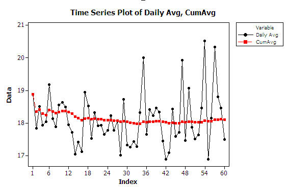
Figure 8.29: Welch plot for high resource configuration
If we run the low resource case of Table 8.13 under the same conditions, an execution error will occur that indicates that the maximum number of entities for the professional version of is exceeded. In this case, the overall arrival rate is too high for the available resources in the model. The samples build up in the queues (especially the input queue) and unprocessed samples will be carried forward each day, eventually building up to a point that exceeds the number of entities permitted. Thus, it should be clear that in the under resourced case the performance measures cannot reach steady state. Whether or not a warm up period is set for these cases, they will naturally be excluded as design alternatives because of exceptionally poor performance. Therefore, setting a warm up period for under capacitated design configurations appears unnecessary. Based on this analysis, a 1 day warm up period will be used to be very conservative across all of the design configurations.
The run setup parameter settings for the initialization bias investigation do not necessarily apply to further experiments. In particular, with the \(3^{rd}\) option, the days are technically within replication data. Option 1 appears to be applicable to future experiments. For option 1, the run length and the number of replications for the experiments need to be determined. The batch means method based on 1 long replication of many days or the method of replication deletion can be utilized in this situation. Because you might want to use the Process Analyzer and possibly OptQuest during the analysis, the method of replication deletion may be more appropriate. Based on the rule of thumb in (Banks et al. 2005), the run length should be at least 10 times the amount of data deleted. Because 1 day of data is being deleted, the run length should be set to 11 days so that a total of 10 days of data will be collected. Now, the number of replications needs to be determined.
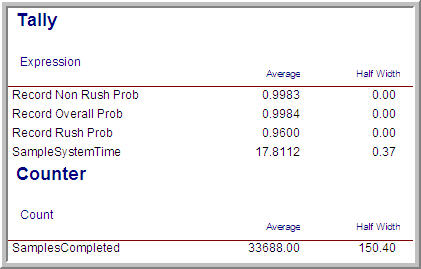
Figure 8.30: User defined results for pilot run
Using the high resource case with 48 sample holders a pilot run was made of 5 replications of 11 days with 1 day warm up. The user-defined results of this run are shown in Figure 8.30. As indicated in the figure, there were a large number of samples completed during each 10 day period and the half-widths of the performance measures are already very acceptable with only 5 replications. Thus, 5 replications will be used in all the experiments that follow. Because other configurations may have more variability and thus require more than 5 replications, a risk is being taken that adequate decisions will be able to be made across all design configurations. Thus, a trade-off is being made between the additional time that pilot runs would entail and the risks associated with making a valid decision.