A.1 Pseudo Random Numbers
This section indicates how uniformly distributed random numbers over the range from 0 to 1 are obtained within simulation programs. While commercial simulation packages provide substantial capabilities for generating random numbers, we still need to understand how this process works for the following reasons:
The random numbers within a simulation experiment might need to be controlled in order to take advantage of them to improve decision making.
In some situations, the commercial package does not have ready made functions for generating the desired random variables. In these situations, you will have to implement an algorithm to generate the random variates.
In addition, simulation is much broader than just using a commercial package. You can perform simulation in any computer language and spreadsheets. The informed modeler should know how the key inputs to simulation models are generated.
In simulation, large amount of cheap (easily computed) random numbers are required. In general, consider how random numbers might be obtained:
Dice, coins, colored balls
Specially designed electronic equipment
Algorithms
Clearly, within the context of computer simulation, it might be best to rely on algorithms; however, if an algorithm is used to generate the random numbers then they will not be truly random. For this reason, the random numbers that are used in computer simulation are called pseudo random.
A set of statistical tests are performed on the pseudo-random numbers generated from algorithms in order to indicate that their properties are not significantly different from a true set of \(U(0,1)\) random numbers. The algorithms that produce pseudo-random numbers are called random number generators. In addition to passing a battery of statistical tests, the random number generators need to be fast and they need to be able to reproduce a sequence of numbers if and when necessary.
The following section discusses random number generation methods. The approach will be practical, with just enough theory to motivate future study of this area and to allow you to understand the important implications of random number generation. A more rigorous treatment of random number and random variable generation can be found such texts as (Fishman 2006) and (Devroye 1986).
A.1.1 Random Number Generators
Over the history of scientific computing, there have been a wide variety of techniques and algorithms proposed and used for generating pseudo-random numbers. A common technique that has been used (and is still in use) within a number of simulation environments is discussed in this text. Some new types of generators that have been recently adopted within many simulation environments, especially the one used within the JSL and Arena, will also be briefly discussed.
A linear congruential generator (LCG) is a recursive algorithm for producing a sequence of pseudo random numbers. Each new pseudo random number from the algorithm depends on the previous pseudo random number. Thus, a starting value called the seed is required. Given the value of the seed, the rest of the sequence of pseudo random numbers can be completely determined by the algorithm. The basic definition of an LCG is as follows
Definition A.2 (Linear Congruential Generator) A LCG defines a sequence of integers, \(R_{0}, R_{1}, \ldots\) between \(0\) and \(m-1\) according to the following recursive relationship:
\[ R_{i+1} = \left(a R_{i} + c\right)\bmod m %) %\left(m\right) \]
where \(R_{0}\) is called the seed of the sequence, \(a\) is called the constant multiplier, \(c\) is called the increment, and \(m\) is called the modulus. \(\left(m, a, c, R_{0}\right)\) are integers with \(a > 0\), \(c \geq 0\), \(m > a\), \(m > c\), \(m > R_{0}\), and \(0 \leq R_{i} \leq m-1\).
To compute a corresponding pseudo-random uniform number, we use
\[ U_{i} = \frac{R_{i}}{m} \]Notice that an LCG defines a sequence of integers and subsequently a sequence of real (rational) numbers that can be considered pseudo random numbers. Remember that pseudo random numbers are those that can “fool” a battery of statistical tests. The choice of the seed, constant multiplier, increment, and modulus, i.e. the parameters of the LCG, will determine the properties of the sequences produced by the generator. With properly chosen parameters, an LCG can be made to produce pseudo random numbers. To make this concrete, let’s look at a simple example of an LCG.
Let’s first remember how to compute using the \(\bmod\) operator. The \(\bmod\) operator is defined as:
\[ z = y \bmod m = y - m \left \lfloor \dfrac{y}{m} \right \rfloor \]
where \(\lfloor x \rfloor\) is the floor operator, which returns the greatest integer that is less than or equal to \(x\). For example,
\[\begin{equation} \begin{split} z & = 17 \bmod 3 \\ & = 17 - 3 \left \lfloor \frac{17}{3} \right \rfloor \\ & = 17 - 3 \lfloor 5.\overline{66} \rfloor \\ & = 17 - 3 \times 5 = 2 \end{split} \end{equation}\]
Thus, the \(\bmod\) operator returns the integer remainder (including zero) when \(y \geq m\) and \(y\) when \(y < m\). For example, \(z = 6 \bmod 9 = 6 - 9 \left\lfloor \frac{6}{9} \right\rfloor = 6 - 9 \times 0 = 6\).
Using the parameters of the LCG, the pseudo-random numbers are:
\[ \begin{split} {R_1} & = (5{R_0} + 1)\bmod 8 = 26\bmod 8 = 2 \Rightarrow {U_1} = 0.25 \\ {R_2} & = (5{R_1} + 1)\bmod 8 = 11\bmod 8 = 3 \Rightarrow {U_2} = 0.375 \\ {R_3} & = (5{R_2} + 1)\bmod 8 = 16\bmod 8 = 0 \Rightarrow {U_3} = 0.0 \\ {R_4} & = (5{R_3} + 1)\bmod 8 = 1\bmod 8 = 1 \Rightarrow {U_4} = 0.125 \\ {R_5} & = 6 \Rightarrow {U_5} = 0.75 \\ {R_6} & = 7 \Rightarrow {U_6} = 0.875 \\ {R_7} & = 4 \Rightarrow {U_7} = 0.5 \\ {R_8} & = 5 \Rightarrow {U_8} = 0.625 \\ {R_9} & = 2 \Rightarrow {U_9} = 0.25 \end{split} \]
In the previous example, the \(U_{i}\) are simple fractions involving \(m = 8\). Certainly, this sequence does not appear very random. The \(U_{i}\) can only take on rational values in the range, \(0,\tfrac{1}{m}, \tfrac{2}{m}, \tfrac{3}{m}, \ldots, \tfrac{(m-1)}{m}\) since \(0 \leq R_{i} \leq m-1\). This implies that if \(m\) is small there will be gaps on the interval \(\left[0,1\right)\), and if \(m\) is large then the \(U_{i}\) will be more densely distributed on \(\left[0,1\right)\).
Notice that if a sequence generates the same value as a previously generated value then the sequence will repeat or cycle. An important property of a LCG is that it has a long cycle, as close to length \(m\) as possible. The length of the cycle is called the period of the LCG. Ideally the period of the LCG is equal to \(m\). If this occurs, the LCG is said to achieve its full period. As can be seen in the example, the LCG is full period. Until recently, most computers were 32 bit machines and thus a common value for \(m\) is \(2^{31} - 1 = 2,147,483,647\), which represents the largest integer number on a 32 bit computer using 2’s complement integer arithmetic. This choice of \(m\) also happens to be a prime number, which leads to special properties.
A proper choice of the parameters of the LCG will allow desirable pseudo random number properties to be obtained. The following result due to (Hull and Dobell 1962), see also (Law 2007), indicates how to check if a LCG will have the largest possible cycle.
Now, let’s apply this theorem to the example LCG and check whether or not it should obtain full period. To apply the theorem, you must check if each of the three conditions holds for the generator.
Condition 1: \(c\) and \(m\) have no common factors other than 1.
The factors of \(m=8\) are \((1, 2, 4, 8)\), since \(c=1\) (with factor 1) condition 1 is true.Condition 2: \((a-1)\) is a multiple of every prime number that divides \(m\). The first few prime numbers are (1, 2, 3, 5, 7). The prime numbers, \(q\), that divide \(m=8\) are \((q =1, 2)\). Since \(a=5\) and \((a-1)=4\), clearly \(q = 1\) divides \(4\) and \(q = 2\) divides \(4\). Thus, condition 2 is true.
Condition 3: If \(4\) divides \(m\), then \(4\) should divide \((a-1)\).
Since \(m=8\), clearly \(4\) divides \(m\). Also, \(4\) divides \((a-1)= 4\). Thus, condition 3 holds.
Since all three conditions hold, the LCG achieves full period.
There are some simplifying conditions, see Banks et al. (2005), which allow for easier application of the theorem. For \(m = 2^{b}\), (\(m\) a power of 2) and \(c\) not equal to 0, the longest possible period is \(m\) and can be achieved provided that \(c\) is chosen so that the greatest common factor of \(c\) and \(m\) is 1 and \(a=4k+1\) where \(k\) is an integer. The previous example LCG satisfies this situation.
For \(m = 2^{b}\) and \(c = 0\), the longest possible period is \((m/4)\) and can be achieved provided that the initial seed, \(R_{0}\) is odd and \(a=8k + 3\) or \(a=8k + 5\) where \(k = 0, 1, 2,\cdots\).
The case of \(m\) a prime number and \(c = 0\), defines a special case of the LCG called a prime modulus multiplicative linear congruential generator (PMMLCG). For this case, the longest possible period is \(m-1\) and can be achieved if the smallest integer, \(k\), such that \(a^{k} -1\) is divisible by \(m\) is \(m-1\).
Thirty-Two bit computers have been very common for over 20 years. In addition, \(2^{31} - 1\) = \(2,147,483,647\) is a prime number. Because of this, \(2^{31} - 1\) has been the choice for \(m\) with \(c=0\). Two common values for the multiplier, \(a\), have been:
\[ \begin{split} a & = 630,360,016\\ a & = 16,807\\ \end{split} \]
The latter of which was used within many simulation packages for a number of years. Notice that for PMMLCG’s the full period cannot be achieved (because \(c=0\)), but with the proper selection of the multiplier, the next best period length of \(m-1\) can be obtained. In addition, for this case \(R_{0} \in \lbrace 1, 2,\ldots , m-1\rbrace\) and thus \(U_{i} \in (0,1)\). The limitation of \(U_{i} \in (0,1)\) is very useful when generating random variables from various probability distributions, since \(0\) cannot be realized. When using an LCG, you must supply a starting seed as an initial value for the algorithm. This seed determines the sequence that will come out of the generator when it is called within software. Since generators cycle, you can think of the sequence as a big circular list as indicated in Figure A.1.
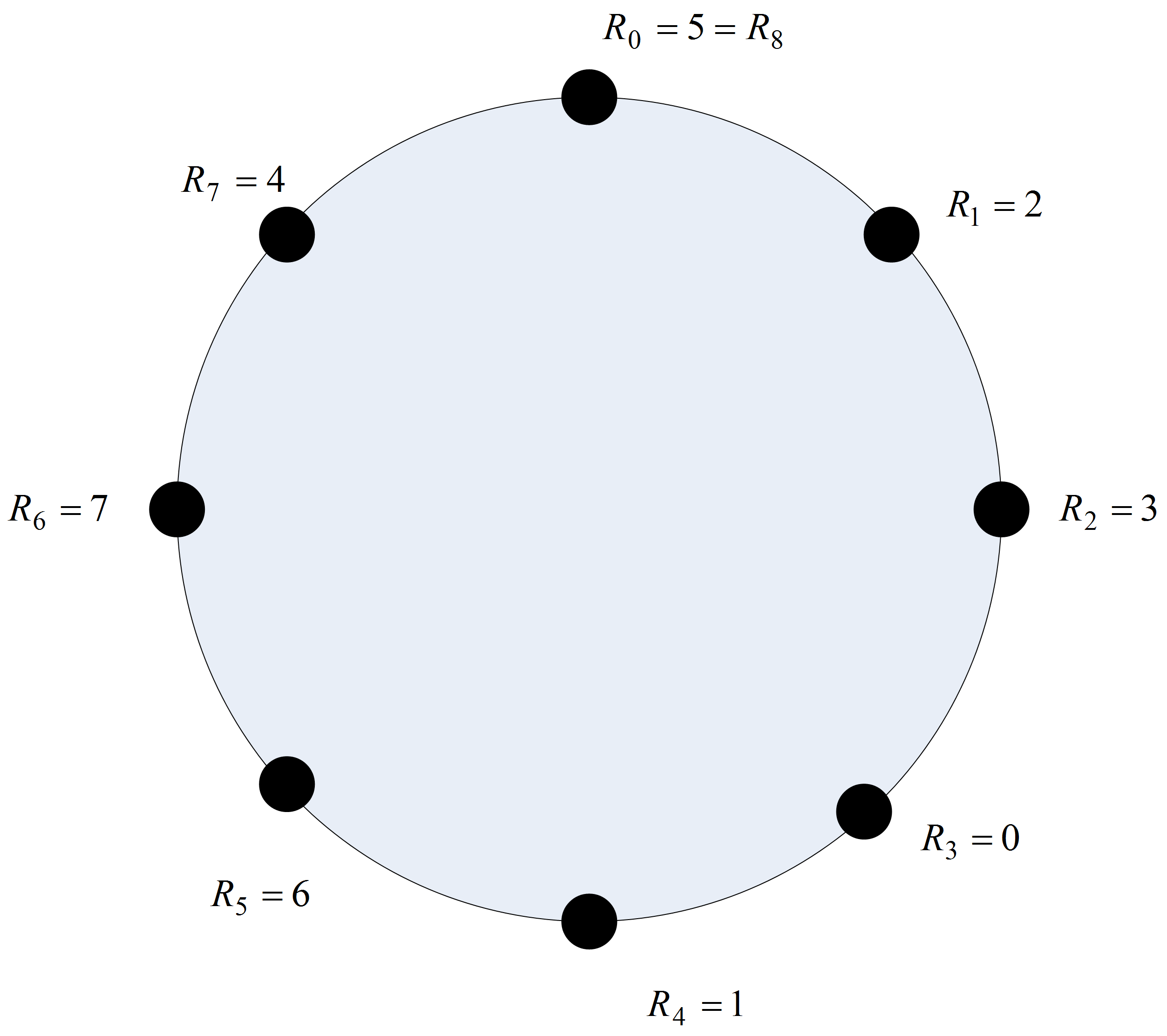
Figure A.1: Sequence for Simple LCG Example
Starting with seed \(R_{0} = 5\), you get a sequence \(\{2, 3, 0, 1, 6, 7, 4, 5\}\). Starting with seed, \(R_{0}=1\), you get the sequence \(\{6, 7, 4, 5, 2, 3, 0, 1\}\). Notice that these two sequences overlap with each other, but that the first half \(\{2, 3, 0, 1\}\) and the second half \(\{6, 7, 4, 5\}\) of the sequence do not overlap. If you only use 4 random numbers from each of these two subsequences then the numbers will not overlap. This leads to the definition of a stream:
You can take the sequence produced by the random number generator and divide it up into subsequences by associating certain seeds with streams. You can call the first subsequence stream 1 and the second subsequence stream 2, and so forth. Each stream can be further divided into subsequences or sub-streams of non-overlapping random numbers.
In this simple example, it is easy to remember that stream 1 is defined by seed, \(R_{0} = 5\), but when \(m\) is large, the seeds will be large integer numbers, e.g. \(R_{0} = 123098345\). It is difficult to remember such large numbers. Rather than remember this huge integer, an assignment of stream numbers to seeds is made. Then, the sequence can be reference by its stream number. Naturally, if you are going to associate seeds with streams you would want to divide the entire sequence so that the number of non-overlapping random numbers in each stream is quite large. This ensures that as a particular stream is used that there is very little chance of continuing into the next stream. Clearly, you want \(m\) to be as large as possible and to have many streams that contain as large as possible number of non-overlapping random numbers. With today’s modern computers even \(m\) is \(2^{31} - 1 = 2,147,483,647\) is not very big. For large simulations, you can easily run through all these random numbers.
Random number generators in computer simulation languages come with a default set of streams that divide the “circle” up into independent sets of random numbers. The streams are only independent if you do not use up all the random numbers within the subsequence. These streams allow the randomness associated with a simulation to be controlled. During the simulation, you can associate a specific stream with specific random processes in the model. This has the advantage of allowing you to check if the random numbers are causing significant differences in the outputs. In addition, this allows the random numbers used across alternative simulations to be better synchronized.
Now a common question for beginners using random number generators can be answered. That is, If the simulation is using random numbers, why to I get the same results each time I run my program? The corollary to this question is, If I want to get different random results each time I run my program, how do I do it? The answer to the first question is that the underlying random number generator is starting with the same seed each time you run your program. Thus, your program will use the same pseudo random numbers today as it did yesterday and the day before, etc. The answer to the corollary question is that you must tell the random number generator to use a different seed (or alternatively a different stream) if you want different invocations of the program to produce different results. The latter is not necessarily a desirable goal. For example, when developing your simulation programs, it is desirable to have repeatable results so that you can know that your program is working correctly. Unfortunately, many novices have heard about using the computer clock to “randomly” set the seed for a simulation program. This is a bad idea and very much not recommended in our context. This idea is more appropriate within a gaming simulation, in order to allow the human gamer to experience different random sequences.
Given current computing power, the previously discussed PMMLCGs are insufficient since it is likely that all the 2 billion or so of the random numbers would be used in performing serious simulation studies. Thus, a new generation of random number generators was developed that have extremely long periods. The random number generator described in L’Ecuyer, Simard, and Kelton (2002) is one example of such a generator. It is based on the combination of two multiple recursive generators resulting in a period of approximately \(3.1 \times 10^{57}\). This is the same generator that is now used in many commercial simulation packages. The generator as defined in (Law 2007) is:
\[ \begin{split} R_{1,i}&=(1,403,580 R_{1,i-2} - 810,728 R_{1,i-3})[\bmod (2^{32}-209)]\\ R_{2,i}&=(527,612R_{2,i-1} - 1,370,589 R_{2,i-3})[\bmod (2^{32}-22,853)]\\ Y_i &=(R_{1,i}-R_{2,i})[\bmod(2^{32}-209)]\\ U_i&=\frac{Y_i}{2^{32}-209} \end{split} \] The generator takes as its initial seed a vector of six initial values \((R_{1,0}, R_{1,1}, R_{1,2}, R_{2,0}, R_{2,1}, R_{2,2})\). The first initially generated value, \(U_{i}\), will start at index \(3\). To produce five pseudo random numbers using this generator we need an initial seed vector, such as: \[\lbrace R_{1,0}, R_{1,1}, R_{1,2}, R_{2,0}, R_{2,1}, R_{2,2} \rbrace = \lbrace 12345, 12345, 12345, 12345, 12345, 12345\rbrace\]
Using the recursive equations, the resulting random numbers are as follows:
| i=3 | i=4 | i=5 | i=6 | i=7 | |||
|---|---|---|---|---|---|---|---|
| \(Z_{1,i-3}=\) | 12345 | 12345 | 12345 | 3023790853 | 3023790853 | ||
| \(Z_{1,i-2}=\) | 12345 | 12345 | 3023790853 | 3023790853 | 3385359573 | ||
| \(Z_{1,i-1}=\) | 12345 | 3023790853 | 3023790853 | 3385359573 | 1322208174 | ||
| \(Z_{2,i-3}=\) | 12345 | 12345 | 12345 | 2478282264 | 1655725443 | ||
| \(Z_{2,i-2}=\) | 12345 | 12345 | 2478282264 | 1655725443 | 2057415812 | ||
| \(Z_{2,i-1}=\) | 12345 | 2478282264 | 1655725443 | 2057415812 | 2070190165 | ||
| \(Z_{1,i}=\) | 3023790853 | 3023790853 | 3385359573 | 1322208174 | 2930192941 | ||
| \(Z_{2,i}=\) | 2478282264 | 1655725443 | 2057415812 | 2070190165 | 1978299747 | ||
| \(Y_i=\) | 545508589 | 1368065410 | 1327943761 | 3546985096 | 951893194 | ||
| \(U_i=\) | 0.127011122076 | 0.318527565471 | 0.309186015655 | 0.82584686312 | 0.221629915834 |
While it is beyond the scope of this text to explore the theoretical underpinnings of this generator, it is important to note that the use of this new generator is conceptually similar to that which has already been described. The generator allows multiple independent streams to be defined along with sub-streams.
The fantastic thing about this generator is the sheer size of the period. Based on their analysis, L’Ecuyer, Simard, and Kelton (2002) state that it will be “approximately 219 years into the future before average desktop computers will have the capability to exhaust the cycle of the (generator) in a year of continuous computing.” In addition to the period length, the generator has an enormous number of streams, approximately \(1.8 \times 10^{19}\) with stream lengths of \(1.7 \times 10^{38}\) and sub-streams of length \(7.6 \times 10^{22}\) numbering at \(2.3 \times 10^{15}\) per stream. Clearly, with these properties, you do not have to worry about overlapping random numbers when performing simulation experiments. The generator was subjected to a rigorous battery of statistical tests and is known to have excellent statistical properties. The subject of modeling and testing different distributions is deferred to a separate part of this book.