6.1 Non-stationary Processes
If a process does not depend on time, it is said to be stationary. When a process depends on time, it is said to be non-stationary. The more formal definitions of stationary/non-stationary are avoided in the discussion that follows.
There are many ways in which you can model non-stationary (time varying) processes in your simulation models. Many of these ways depend entirely on the system being studied and through that study appropriate modeling methods will become apparent. For example, suppose that workers performing a task learn how to more efficiently perform the task every time that they repeat the task. The task time will depend on the time (number of previously performed tasks). For this situation, you might use a learning curve model as a basis for changing the task times as the number of repetitions of the task increases.
As another example, suppose the worker’s availability depends on a schedule, such as having a 30-minute break after accumulating so much time. In this situation, the system’s resources are dependent on time. Modeling this situation is described later in this chapter.
Let’s suppose that the following situation needs to be modeled. Workers are assigned a shift of 8 hours and have a quota to fill. Do you think that it is possible that their service times would, on average, be less during the latter part of the shift? Sure. They might work faster in order to meet their quota during the latter part of the shift. If you did not suspect this phenomenon and performed a time study on the workers in the morning and fit a distribution to these data, you would be developing a distribution for the service times during the morning. If you applied this distribution to the entire shift, then you may have a problem matching your simulation throughput numbers to the real throughput.
As you can see, if you suspect that a non-stationary process is involved, then it is critical that you also record the time that the observation was made. The time series plot that was discussed for input modeling helps in assessing non-stationary behavior; however, it only plots the order in which the data were collected. If you collect 25 observations of the service time every morning, you might not observe non-stationary behavior. To observe non-stationary behavior it is important to collect observations across periods of time.
One way to better plan your observations is to randomize when you will take the observations. Work sampling methods often require this. The day is divided into intervals of time and the intervals randomly selected in which to record an activity. By comparing the behavior of the data across the intervals, you can begin to assess whether time matters in the modeling as demonstrated in Section B.3.1. Even if you do not divide time into logical intervals, it is good practice to record the date and time for each of the observations that you make so that the observations can later be placed into logical intervals. As you may now be thinking, modeling a non-stationary process will take a lot of care and more observations than a stationary process.
A very common non-stationary process that you have probably experienced is a non- stationary arrival process. In a non-stationary arrival process, the arrival process to the system will vary by time (e.g., by hour of the day). Because the arrival process is a key input to the system, the system will thus become non-stationary. For example, in the drive-through pharmacy example, the arrival of customers occurred according to a Poisson process with mean rate \(\lambda\) per hour.
As a reminder, \(\lambda\) represents the mean arrival rate or the expected number of customers per unit time. Suppose that the expected arrival rate is five per hour. This does not mean that the pharmacy will get five customers every hour, but rather that on average five customers will arrive every hour. Some hours will get more than five customers and other hours will get less. The implication for the pharmacy is that they should expect about five per hour (every hour of the day) regardless of the time of day. Is this realistic? It could be, but it is more likely that the mean number of arriving customers will vary by time of day. For example, would you expect to get five customers per hour from 4 a.m. to 5 a.m., from 12 noon to 1 p.m., from 4 p.m. to 6 p.m.? Probably not! A system like the pharmacy will have peaks and valleys associated with the arrival of customers. Thus, the mean arrival rate of the customers may vary with the time of day. That is, \(\lambda\) is really a function of time, \(\lambda(t)\).
To more realistically model the arrival process to the pharmacy, you need to model a non-stationary arrival process. Let’s think about how data might be collected in order to model a non-stationary arrival process. First, as in the previous service time example, you need to think about dividing the day into logical periods of time. A pilot study may help in assessing how to divide time, or you might simply pick a convenient time division such as hours. You know that the CREATE module requires a distribution that represents the time between arrivals. Ideally, you should collect the time of every arrival, \(T_i\), throughout the day. Then, you can take the difference among consecutive arrivals, \(T_i - T_{i-1}\) and fit a distribution to the inter-arrival times. Looking at the \(T_i\) over time may help to assess whether you need different distributions for different time periods during the day. Suppose that you do collect the observations and find that three different distributions are reasonable models given the following data:
Exponential, \(E[X] = 60\), for midnight to 8 a.m.
Lognormal, \(E[X] = 12\), \(Var[X] = 4\), for 8 a.m. to 4 p.m.
Triangular, min = 10; mode = 16; max = 20, for 4 p.m. to midnight
One simple method for implementing this situation is to CREATE a logical entity that selects the appropriate distribution for the current time. In other words, schedule a logical entity to arrive at midnight so that the time between arrival distribution can be set to exponential, schedule an entity to arrive at 8 a.m. to switch to lognormal, and schedule an entity to arrive at 4 p.m. to switch to triangular. This can easily be accomplished by holding the distributions within an arrayed expression and using a clock entity to determine which period of time is active and indexing into the arrayed expression accordingly. Clearly, this varies the arrival process in a time-varying manner. There is nothing wrong with this modeling approach if it works well for the situation. In taking such an approach, you need a lot of data. Not only do you need to record the time of every arrival, but you need enough arrivals in order to adequately fit distributions to the time between events for various time periods. This may or may not be feasible in practice.
Often in modeling arrival processes, you cannot readily collect the actual times of the arrivals. If you can, you should try, but sometimes you just cannot. Instead, you are limited to a count of the number of arrivals in intervals of time. For example, a computer system records the number of people arriving every hour but not their individual arrival times. This is not uncommon since it is much easier to store summary counts than it is to store all individual arrival times. Suppose that you had count data as shown in Table 6.1.
| Interval | Mon | Tue | Wed | Thurs | Fri | Sat | Sun |
|---|---|---|---|---|---|---|---|
| 12 am – 6 am | 3 | 2 | 1 | 2 | 4 | 2 | 1 |
| 6 am - 9 am | 6 | 4 | 6 | 7 | 8 | 7 | 4 |
| 9 am - 12 pm | 10 | 6 | 4 | 8 | 10 | 9 | 5 |
| 12 pm - 2 pm | 24 | 25 | 22 | 19 | 26 | 27 | 20 |
| 2 pm - 5 pm | 10 | 16 | 14 | 16 | 13 | 16 | 15 |
| 5 pm - 8 pm | 30 | 36 | 26 | 35 | 33 | 32 | 18 |
| 8 pm - 12 am | 14 | 12 | 8 | 13 | 12 | 15 | 10 |
Of course, how the data are grouped into intervals will affect how the data can be modeled. Grouping is part of the modeling process. Let’s accept these groups as appropriate for this situation. Looking at the intervals, you see that more arrivals tend to occur from 12 pm to 2 pm and from 5 pm to 8 pm. As discussed in Section B.3.1, we could test for this non-stationary behavior and check if the counts depend on the time of day. It is pretty clear that this is the case for this situation. Perhaps this corresponds to when people who visit the pharmacy can get off of work. Clearly, this is a non-stationary situation. What kinds of models can be used for this type of count data?
A simple and often reasonable approach to this situation is to check whether the number of arrivals in each interval occurs according to a Poisson distribution. If so, then you know that the time between arrivals in an interval is exponential. When you can divide time so that the number of events in the intervals is Poisson (with different mean rates), then you can use a non-stationary or non-homogeneous Poisson process as the arrival process.
Consider the first interval to be 12 am to 6 am; to check if the counts are Poisson in this interval, there are seven data points (one for every day of the week for the given period). This is not a lot of data to use to perform a chi-square goodness-of-fit test for the Poisson distribution. So, to do a better job at modeling the situation, many more days of data are needed. The next question is: Are all the days the same? It looks like Sunday may be a little different than the rest of the days. In particular, the counts on Sunday appear to be a little less on average than the other days of the week. In this situation, you should also check whether the day of the week matters to the counts. As we illustrated in Section B.3.1, one method of doing this is to perform a contingency table test.
Let’s assume for simplicity that there is not enough evidence to suggest that the days are different and that the count data in each interval is well modeled with a Poisson distribution. In this situation, you can proceed with using a non-stationary Poisson process. From the data you can calculate the average arrival rate for each interval and the rate per hour for each interval as shown in Table 6.2. In the table, 2.14 is the average of the counts across the days for the interval 12 am to 6 pm. In the rate per hour column, the interval rate has been converted to an hourly basis by dividing the rate for the interval by the number of hours in the interval. Figure 6.1 illustrates the time-varying behavior of the mean arrival rates over the course of a day.
| Interval | Avg. | Length (hrs) | Rate per hour |
|---|---|---|---|
| 12 am – 6 am | 2.14 | 6 | 0.36 |
| 6 am - 9 am | 6.0 | 3 | 2.0 |
| 9 am - 12 pm | 7.43 | 3 | 2.48 |
| 12 pm - 2 pm | 23.29 | 2 | 11.645 |
| 2 pm - 5 pm | 14.29 | 3 | 4.76 |
| 5 pm - 8 pm | 30.0 | 3 | 10 |
| 8 pm - 12 am | 12.0 | 4 | 3.0 |
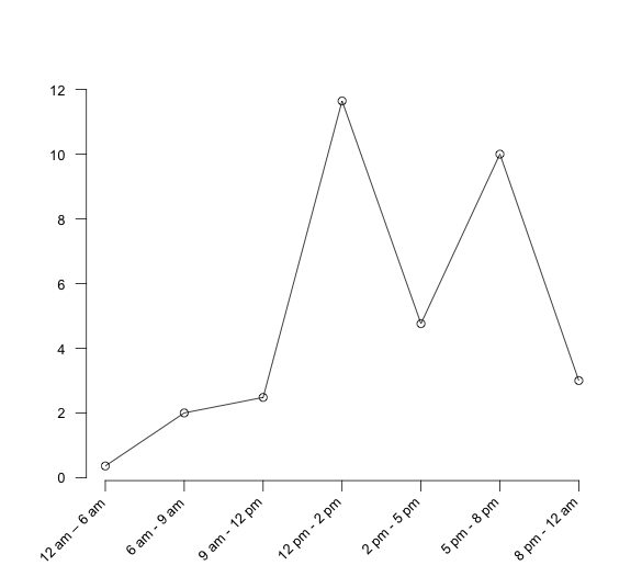
Figure 6.1: Arrival rate per hour for time intervals
The two major methods by which a non-stationary Poisson process can be generated are thinning and rate inversion. Both methods will be briefly discussed; however, the interested reader is referred to (L. M. Leemis and Park 2006) or (Ross 1997) for more of the theory underlying these methods. Before these methods are discussed, it is important to point out that the naive method of using different Poisson processes for each interval and subsequently different exponential distributions to represent the inter-arrival times could be used to model this situation by switching the distributions as previously discussed. However, the switching method is not technically correct for generating a non-stationary Poisson process. This is because it will not generate a non-stationary Poisson process with the correct probabilistic underpinnings. Thus, if you are going to model a process with a non-stationary Poisson process, you should use either thinning or rate inversion to be technically correct.
6.1.1 Thinning Method
For the thinning method, a stationary Poisson process with a constant rate,\(\lambda^{*}\), and arrival times, \(t_{i}^{*}\), is first generated, and then potential arrivals, \(t_{i}^{*}\), are rejected with probability:
\[p_r = 1 - \frac{\lambda(t_{i}^{*})}{\lambda^{*}}\]
where \(\lambda(t)\) is the mean arrival rate as a function of time. Often, \(\lambda^{*}\) is set as the maximum arrival rate over the time horizon, such as:
\[\lambda^{*} = \max\limits_{t} \lbrace \lambda(t) \rbrace\]
In the example, \(\lambda^{*}\) would be the mean of the 5 pm to 8 pm interval, \(\lambda^{*} = 11.645\). The following pseudo-code for implementing the thinning method creates entities at the maximum rate and thins them according to which period is currently active.
DECIDE with chance, \(1 - \frac{\lambda(t_{i}^{*})}{\lambda^{*}}\)
IF accepted THEN
Go to Label B
ELSE
DISPOSE
END IF
END DECIDE
B: enter model and use arrival
An array stores each arrival rate for the intervals, and a variable is used to hold the maximum arrival rate over the time horizon. To implement the arrival rate function, the code creates a logical entity that keeps track of the current interval as a variable that can be used to index the array of arrival rates. If the simulation lasts past the time horizon of the arrival rate function, then the variable that keeps track of the interval should be reset to start counting from the first period.
A: ASSIGN vPeriod = vPeriod + 1
DECIDED IF vPeriod < vNumPeriods THEN
DELAY for period length
ELSE
vPeriod = 0
END DECIDE
GO TO Label A:
One of the exercises in this chapter requires implementing the thinning algorithm in . The theoretical basis for why thinning works can be found in (Ross 1997).
6.1.2 Rate Inversion Method
The second method for generating a non-stationary Poisson process is through the rate inversion algorithm. In this method, a \(\lambda = 1\) Poisson process is generated, and the inverse of the mean arrival rate function is used to re-scale the times of arrival to the appropriate scale. This section does not discuss the theory behind this algorithm. Instead, see (L. M. Leemis and Park 2006) for further details of the theory, fitting, and the implementation of this method in simulation. This method is available for piece-wise constant-rate functions in by using an Arrivals Schedule associated with a CREATE module. Let’s see how to implement the example using an Arrivals Schedule.
The following is available in the file PharmacyModelNSPP.doe that accompanies this chapter. The first step in implementing a non-stationary Poisson process in is to define the intervals and compute the rates per hour as per Table 6.2. It is extremely important to have the rates on a per hour basis. The SCHEDULE module is a data module on the Basic Process panel.
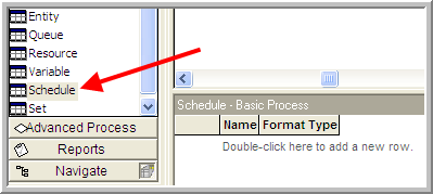
Figure 6.2: SCHEDULE data module
Figure 6.2 illustrates where to find the SCHEDULE in the Basic Process panel. To use the SCHEDULE module, double-click on the data module area to add a new schedule. Schedules can be of type Capacity, Arrival, and Other. Right-clicking on the row and using Edit via Dialog will give you the SCHEDULE dialog window. The text boxes for the SCHEDULE dialog follow:
- Format Type
Schedules can be defined as a collection of value, duration pairs (Duration) or they can be defined using the calendar editor. The calendar editor allows for the input of a complex schedule that can be best described by a Gregorian calendar (i.e., days, months, etc.).
- Type
Capacity refers to time varying schedules for resources. Arrival refers to non- stationary Poisson arrivals. Other can be used to represent other types of time delayed schedules.
- Time Units
This field represents how the time units for the durations will be interpreted. The field only refers to the durations, not the arrival rates.
- Scale Factor
This field can be used to easily change all the values in the duration value pairs.
- Durations
The length of time of the interval for the associated value. Once all the durations have been executed, the schedule will repeat unless the last duration is left infinite.
- Value
This field represents either the capacity to be used for the resource or the arrival rate (in entities per hour), depending on which type of schedule was specified.
- Name
Name of the module.
The SCHEDULE module offers a number of ways in which to enter the information required for the schedule. The most straightforward method is to enter each value and duration pair using the Add button on the dialog box. You will be prompted for each pair. In this case, the arrival rate (per hour) and the duration that the arrival rate will last should be entered. The completed dialog entries are shown in Figure 6.3.
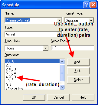
Figure 6.3: SCHEDULE dialog
Note that the arrival rates are given per hour. Not entering the arrival rates per hour is a common error in using this module. Even if you specify the time units of the dialog as minutes, the arrival rates must be per hour. The time units only refer to the duration values. The duration values can also be entered using a spreadsheet like view.
Once the schedule has been defined, the last step is to indicate in the CREATE module that it should use the SCHEDULE. This is shown in Figure 6.4 where the Time Between Arrivals Type has been specified as Schedule with the appropriate Schedule Name. The schedule as in Figure 6.3 shows that the duration values add up to 24 hours so that a full day’s worth of arrival rates are specified. If you simulate the system for more than one day, what will happen on the second day? Because the schedule has a duration, value pair for each interval, the schedule will repeat after the last duration occurs. If the schedule is specified with an infinite last duration, the value specified will be used for the rest of the simulation and the schedule will not repeat.
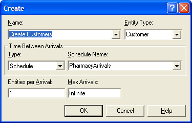
Figure 6.4: CREATE module with schedule type
As indicated in this limited example, it is relatively easy to model a non-stationary Poisson arrival process within Arena. If the arrival process to the system is non-stationary, then it is probably a good idea to vary the resources available in they system according to the arrival pattern. The next section discusses how to extend the modeling of resources to include time varying behavior as well as the ability to fail at random points in time.