C.1 Single Line Queueing Stations
Chapter 2 presented the pharmacy model and analyzed it with a single server, single queue queueing system called the M/M/1. This section shows how the formulas for the M/M/1 model in Chapter 2 were derived and discusses the key notation and assumptions of analytical models for systems with a single queue. In addition, you will also learn how to simulate variations of these models.
In a queueing system, there are customers that compete for resources by moving through processes. The competition for resources causes waiting lines (queues) to form and delays to occur within the customer’s process. In these systems, the arrivals and/or service processes are often stochastic. Queueing theory is a branch of mathematical analysis of systems that involve waiting lines in order to predict (and control) their behavior over time. The basic models within queueing theory involve a single line that is served by a set of servers. Figure C.1 illustrates the major components of a queueing system with a single queue feeding into a set of servers.
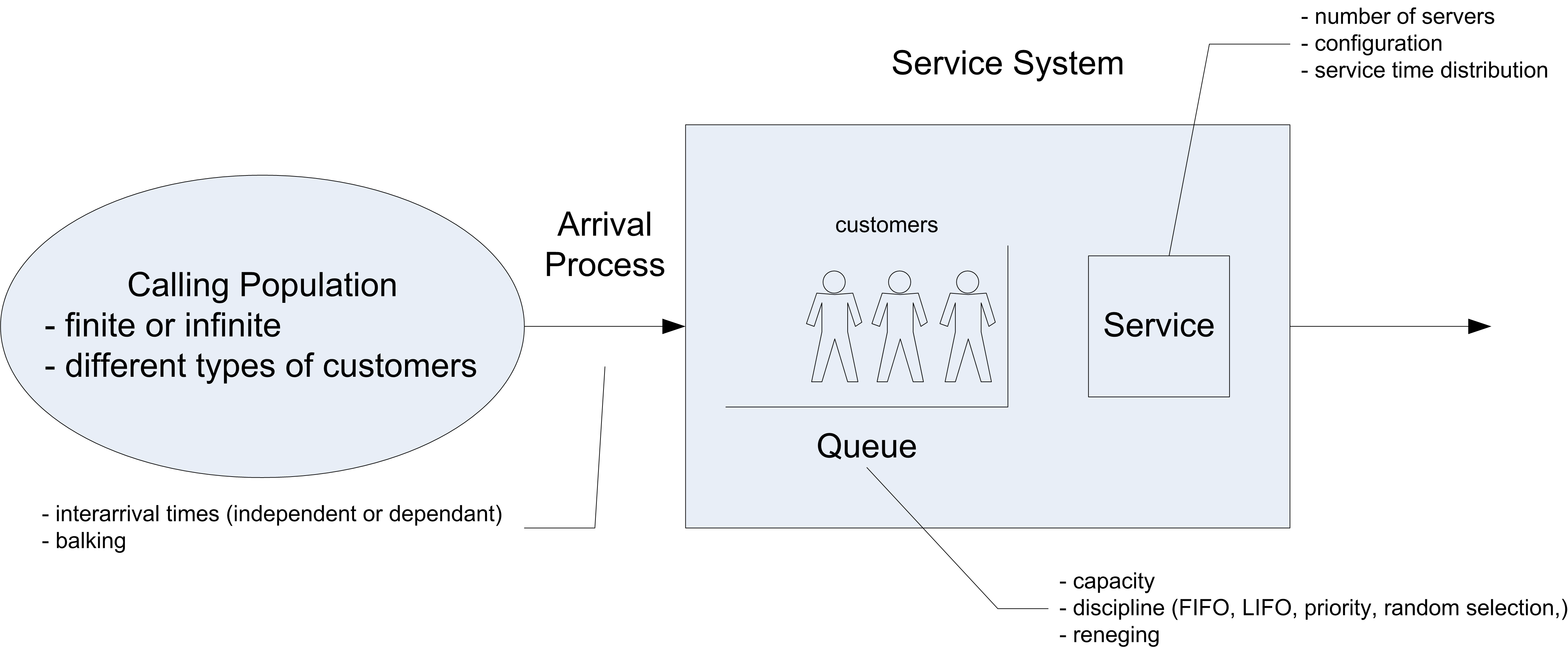
Figure C.1: Example single queue system
In queueing theory the term customer is used as a generic term to describe the entities that flow and receive service. A resource is a generic term used to describe the components of the system that are required by a customer as the customer moves through the system. The individual units of the resource are often called servers. In Figure C.1, the potential customers can be described as coming from a calling population. The term calling population comes from the historical use of queueing models in the analysis of phone calls to telephone trunk lines. Customers within the calling population may arrive to the system according to an arrival process. In the finite population case, the arrival rate that the system experiences will quite naturally decrease as customers arrive since fewer customers are available to arrive if they are within the system.
In the infinite calling population case, the rate of arrivals to the system does not depend upon on how many customers have already arrived. In other words, there are so many potential customers in the population that the arrival rate to the system is not affected by the current number of customers within the system. Besides characterizing the arrival process by the rate of arrivals, it is useful to think in terms of the inter-arrival times and in particular the inter-arrival time distribution. In general, the calling population may also have different types of customers that arrive at different rates. In the analytical analysis presented here, there will only be one type of customer.
The queue is that portion of the system that holds waiting customers. The two main characteristics for the queue are its size or capacity, and its discipline. If the queue has a finite capacity, this indicates that there is only enough space in the queue for a certain number of customers to be waiting at any given time. The queue discipline refers to the rule that will be used to decide the order of the customers within the queue. A first-come, first-served (FCFS) queue discipline orders the queue by the order of arrival, with the most recent arrival always joining the end of the queue. A last-in, first out (LIFO) queue discipline has the most recent arrival joining the beginning of the queue. A last-in, first out queue discipline acts like a stack of dishes. The first dish is at the bottom of the stack, and the last dish added to the stack is at the top of the stack. Thus, when a dish is needed, the next dish to be used is the last one added to the stack. This type of discipline often appears in manufacturing settings when the items are placed in bins, with newly arriving items being placed on top of items that have previously arrived.
Other disciplines include random and priority. You can think of a random discipline modeling the situation of a server randomly picking the next part to work on (e.g. reaches into a shallow bin and picks the next part). A priority discipline allows the customers to be ordered within the queue by a specified priority or characteristic. For example, the waiting items may be arranged by due-date for a customer order.
The resource is that portion of the system that holds customers that are receiving service. Each customer that arrives to the system may require a particular number of units of the resource. The resource component of this system can have 1 or more servers. In the analytical treatment, each customer will required only one server and the service time will be governed by a probability distribution called the service time distribution. In addition, for the analytical analysis the service time distribution will be the same for all customers. Thus, the servers are all identical in how they operate and there is no reason to distinguish between them. Queueing systems that contain servers that operate in this fashion are often referred to as parallel server systems. When a customer arrives to the system, the customer will either be placed in the queue or placed in service. After waiting in line, the customer must select one of the (identical) servers to receive service. The following analytical analysis assumes that the only way for the customer to depart the system is to receive service.
C.1.1 Queueing Notation
The specification of how the major components of the system operate gives a basic system configuration. To help in classifying and identifying the appropriate modeling situations, Kendall’s notation ((Kendall 1953)) can be used. The basic format is:
arrival process / service process / number of servers / system capacity / size of the calling population / queue discipline
For example, the notation M/M/1 specifies that the arrival process is Markovian (M) (exponential time between arrivals), the service process is Markovian (M) (exponentially distributed service times, and that there is 1 server. When the system capacity is not specified it is assumed to be infinite. Thus, in this case, there is a single queue that can hold any customer that arrives. The calling population is also assumed to be infinite if not explicitly specified. Unless otherwise noted the queue discipline is assumed to be FCFS.
Traditionally, the first letter(s) of the appropriate distribution is used to denote the arrival and service processes. Thus, the case LN/D/2 represents a queue with 2 servers having a lognormally (LN) distributed time between arrivals and deterministic (D) service times. Unless otherwise specified it is typically assumed that the arrival process is a renewal process, i.e. that the time between arrivals are independent and identically distributed and that the service times are also independent and identically distributed.
Also, the standard models assume that the arrival process is independent of the service process and vice a versa. To denote any distribution, the letter G for general (any) distribution is used. The notation (GI) is often used to indicate a general distribution in which the random variables are independent. Thus, the G/G/5 represents a queue with an arrival process having any general distribution, a general distribution for the service times, and 5 servers. Figure C.2 illustrates some of the common queueing systems as denoted by Kendall’s notation.
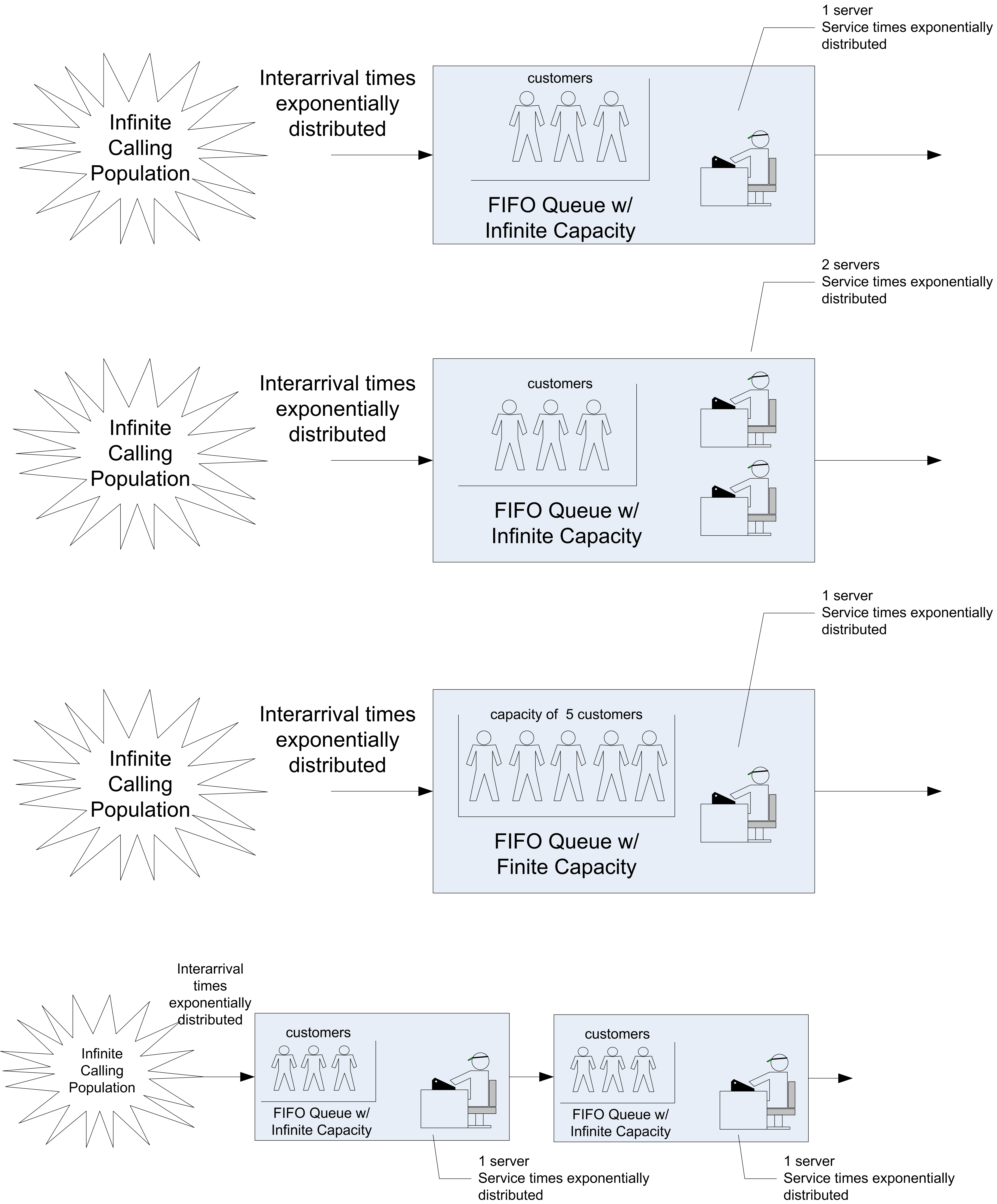
Figure C.2: Illustrating some common queueing situations
There are a number of quantities that form the basis for measuring the performance of queueing systems: - The time that a customer spends waiting in the queue: \(T_q\)
The time that a customer spends in the system (queue time plus service time): \(T\)
The number of customers in the queue at time \(t\): \(N_q(t)\)
The number of customers that are in the system at time t: \(N(t)\)
The number of customer in service at time \(t\): \(N_b(t)\)
These quantities will be random variables when the queueing system has stochastic elements. We will assume that the system is work conserving, i.e. that the customers do not exit without received all of their required service and that a customer uses one and only one server to receive service. For a work conserving queue, the following is true:
\[N(t) = N_q(t) + N_b(t)\]
This indicates that the number of customers in the system must be equal to the number of customers in queue plus the number of customers in service. Since the number of servers is known, the number of busy servers can be determined from the number of customers in the system. Under the assumption that each customer requires 1 server (1 unit of the resource), then \(N_b(t)\) is also the current number of busy servers. For example, if the number of servers is 3 and the number of customers in the system is 2, then there must be 2 customers in service (two servers that are busy). Therefore, knowledge of \(N(t)\) is sufficient to describe the state of the system. Because \(N(t) = N_q(t) + N_b(t)\) is true, the following relationship between expected values is also true:
\[E[N(t)] = E[N_q(t)] + E[N_b(t)]\]
If \(\mathit{ST}\) is the service time of an arbitrary customer, then it should be clear that:
\[E[T] = E[T_q] + E[\mathit{ST}]\]
That is, the expected system time is equal to the expected waiting time in the queue plus the expected time spent in service.
C.1.2 Little’s Formula
Chapter 3 presented time persistent data and computed time-averages. For queueing systems, one can show that relationships exist between such quantities as the expected number in the queue and the expected waiting time in the queue. To understand these relationships, consider Figure C.3 which illustrates the sample path for the number of customers in the queue over a period of time.
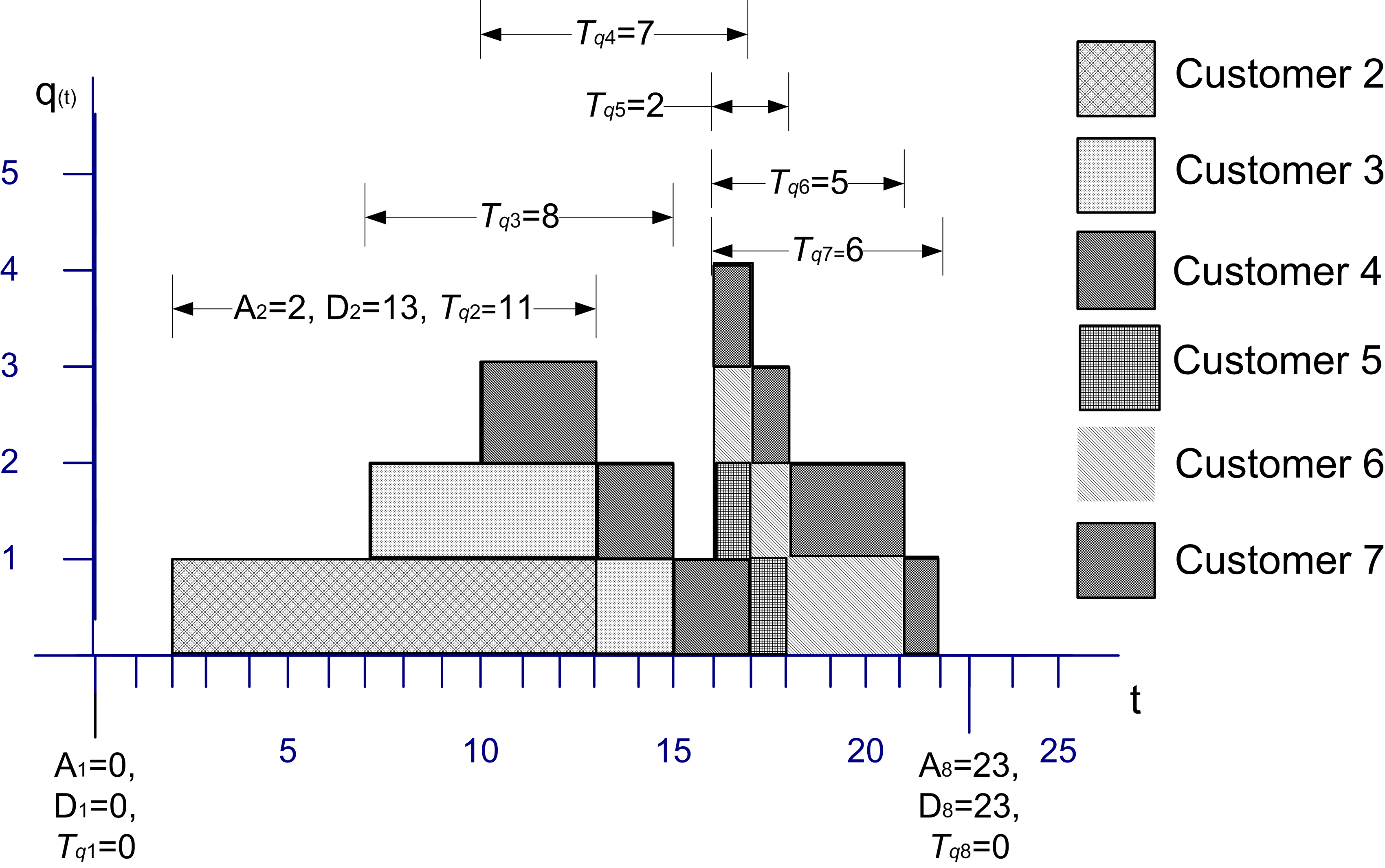
Figure C.3: Sample path for the number of customers in a queue
Let \(A_i; i = 1 \ldots n\) represent the time that the \(i^{th}\) customer enters the queue, \(D_i; i = 1 \ldots n\) represent the time that the \(i^{th}\) customer exits the queue, and \(T_{q_i}\) = \(D_i\) - \(A_i\) for \(i = 1 \ldots n\) represent the time that the \(i^{th}\) customer spends in the queue. Recall that the average time spent in the queue was:
\[\bar{T}_q = \frac{\sum_{i=1}^n T_{q_i}}{n} =\frac{0 + 11 + 8 + 7 + 2 + 5 + 6 + 0}{8} = \frac{39}{8} = 4.875\]
The average number of customers in the queue was:
\[\begin{aligned} \bar{L}_q & = \frac{0(2-0) + 1(7-2) + 2(10-7) + 3(13-10) + 2(15-13) + 1(16-15)}{25}\\ & + \frac{4(17-16) + 3(18-17) + 2(21-18) + 1(22-21) + 0(25-22)}{25} \\ & = \frac{39}{25} = 1.56\end{aligned}\]
By considering the waiting time lengths within the figure, the area under the sample path curve can be computed as:
\[\sum_{i=1}^n T_{q_i} = 39\]
But, by definition the area should also be:
\[\int_{t_0}^{t_n} q(t)\mathrm{d}t\]
Thus, it is no coincidence that the computed value for the numerators in \(\bar{T}_q\) and \(\bar{L}_q\) for the example is 39. Operationally, this must be the case.
Define \(\bar{R}\) as the average rate that customers exit the queue. The average rate of customer exiting the queue can be estimated by counting the number of customers that exit the queue over a period of time. That is,
\[\bar{R} = \frac{n}{t_n - t_0}\]
where \(n\) is the number of customers that departed the system during the time \(t_n - t_0\). This quantity is often called the average throughput rate. For this example, \(\bar{R}\) = 8/25. By combining these equations, it becomes clear that the following relationship holds:
\[\bar{L}_q = \frac{\int\limits_{t_0}^{t_n} q(t)\mathrm{d}t}{t_n - t_0} = \frac{n}{t_n - t_0} \times \frac{\sum_{i=1}^n T_{q_i}}{n} = \bar{R} \times \bar{T}_q\]
This relationship is a conservation law and can also be applied to other portions of the queueing system as well. In words the relationship states that:
Average number in queue = average throughput rate \(\times\) average waiting time in queue
When the service portion of the system is considered, then the relationship can be translated as:
Average number in service = average throughput rate \(\times\) average time in service
When the entire queueing system is considered, the relationship yields:
Average number in the system = average throughput rate \(\times\) average time in the system
These relationships hold operationally for these statistical quantities as well as for the expected values of the random variables that underlie the stochastic processes. This relationship is called Little’s formula after the queueing theorist who first formalized the technical conditions of its applicability to the stochastic processes within queues of this nature. The interested reader is referred to (Little 1961) and (Glynn and Whitt 1989) for more on these relationships. In particular, Little’s formula states a relationship between the steady state expected values for these processes.
To develop these formulas, define \(N\), \(N_q\), \(N_b\) as random variables that represent the number of customers in the system, in the queue, and in service at an arbitrary point in time in steady state. Also, let \(\lambda\) be the expected arrival rate so that \(1/\lambda\) is the mean of the inter-arrival time distribution and let \(\mu = 1/E[\mathit{ST}]\) so that \(E[\mathit{ST}] = 1/\mu\) is the mean of the service time distribution. The expected values of the quantities of interest can be defined as:
\[\begin{aligned} L & \equiv E[N] \\ L_q & \equiv E[N_q]\\ B & \equiv E[N_b]\\ W & \equiv E[T] \\ W_q & \equiv E[T_q]\end{aligned}\]
Thus, it should be clear that
\[\begin{aligned} L & = L_q + B \\ W & = W_q + E[\mathit{ST}]\end{aligned}\]
In steady state, the mean arrival rate to the system should also be equal to the mean through put rate. Thus, from Little’s relationship the following are true:
\[\begin{aligned} L & = \lambda W \\ L_q & = \lambda W_q\\ B & = \lambda E[\mathit{ST}] = \frac{\lambda}{\mu}\end{aligned}\]
To gain an intuitive understanding of Little’s formulas in this situation, consider that in steady state the mean rate that customers exit the queue must also be equal to the mean rate that customers enter the queue. Suppose that you are a customer that is departing the queue and you look behind yourself to see how many customers are left in the queue. This quantity should be \(L_q\) on average. If it took you on average \(W_q\) to get through the queue, how many customers would have arrived on average during this time? If the customers arrive at rate \(\lambda\) then \(\lambda\) \(\times\) \(W_q\) is the number of customers (on average) that would have arrived during your time in the queue, but these are the customers that you would see (on average) when looking behind you. Thus, \(L_q = \lambda W_q\).
Notice that \(\lambda\) and \(\mu\) must be given and therefore \(B\) is known. The quantity \(B\) represents the expected number of customers in service in steady state, but since a customer uses only 1 server while in service, \(B\) also represents the expected number of busy servers in steady state. If there are \(c\) identical servers in the resource, then the quantity, \(B/c\) represents the fraction of the servers that are busy. This quantity can be interpreted as the utilization of the resource as a whole or the average utilization of a server, since they are all identical. This quantity is defined as:
\[\rho = \frac{B}{c} = \frac{\lambda}{c \mu}\]
The quantity, \(c\mu\), represents the maximum rate at which the system can perform work on average. Because of this \(c\mu\) can be interpreted as the mean capacity of the system. One of the technical conditions that is required for Little’s formula to be applicable is that \(\rho < 1\) or \(\lambda < c \mu\). That is, the mean arrival rate to the system must be less than mean capacity of the system. This also implies that the utilization of the resource must be less than 100%.
The queueing system can also be characterized in terms of the offered load. The offered load is a dimensionless quantity that gives the average amount of work offered per time unit to the \(c\) servers. The offered load is defined as: \(r = \lambda/\mu\). Notice that this can be interpreted as each customer arriving with \(1/\mu\) average units of work to be performed. The steady state conditions thus indicate that \(r < c\). In other words, the arriving amount of work to the queue cannot exceed the number of servers. These conditions make sense for steady state results to be applicable, since if the mean arrival rate was greater than the mean capacity of the system, the waiting line would continue to grow over time.
C.1.3 Deriving Formulas for Markovian Single Queue Systems
Notice that with \(L = \lambda W\) and the other relationships, all of the major performance measures for the queue can be computed if a formula for one of the major performance measures (e.g. \(L\), \(L_q\), \(W\), or \(W_q\)) are available. In order to derive formulas for these performance measures, the arrival and service processes must be specified.
This section shows that for the case of exponential time between arrivals and exponential service times, the necessary formulas can be derived. It is useful to go through the basic derivations in order to better understand the interpretation of the various performance measures, the implications of the assumptions, and the concept of steady state.
To motivate the development, let’s consider a simple example. Suppose you want to model an old style telephone booth, which can hold only one person while the person uses the phone. Also assume that any people that arrive while the booth is in use immediately leave. In other words, nobody waits to use the booth.
For this system, it is important to understand the behavior of the stochastic process \(N(t); t \geq 0\), where \(N(t)\) represents the number of people that are in the phone booth at any time \(t\). Clearly, the possible values of \(N(t)\) are 0 and 1, i.e. \(N(t) \in \lbrace 0, 1 \rbrace\). Developing formulas for the probability that there are 0 or 1 customers in the booth at any time \(t\), i.e. \(P_i(t) = P\lbrace N(t) = i\rbrace\) will be the key to modeling this situation.
Let \(\lambda\) be the mean arrival rate of customers to the booth and let \(\mathit{ST} = 1/\mu\) be the expected length of a telephone call. For example, if the mean time between arrivals is 12 minutes, then \(\lambda\) = 5/hr, and if the mean length of a call is 10 minutes, then \(\mu\) = 6/hr. The following reasonable assumptions will be made:
The probability of a customer arriving in a small interval of time, \(\Delta t\), is roughly proportional to the length of the interval, with the proportionality constant equal to the mean rate of arrival, \(\lambda\).
The probability of a customer completing an ongoing phone call during a small interval of time is roughly proportional to the length of the interval and the proportionality constant is equal to the mean service rate, \(\mu\).
The probability of more than one arrival in an arbitrarily small interval, \(\Delta t\), is negligible. In other words, \(\Delta t\), can be made small enough so that only one arrival can occur in the interval.
The probability of more than one service completion in an arbitrarily small interval, \(\Delta t\), is negligible. In other words, \(\Delta t\), can be made small enough so that only one service can occur in the interval.
Let \(P_0(t)\) and \(P_1(t)\) represent the probability that there is 0 or 1 customer using the booth, respectively. Suppose that you observe the system at time \(t\) and you want to derive the probability for 0 customers in the system at some future time, \(t + \Delta t\). Thus, you want, \(P_0(t + \Delta t)\).
For there to be zero customers in the booth at time \(t + \Delta t\), there are two possible situations that could occur. First, there could have been no customers in the system at time \(t\) and no arrivals during the interval \(\Delta t\), or there could have been one customer in the system at time \(t\) and the customer completed service during \(\Delta t\). Thus, the following relationship should hold:
\[\begin{aligned} \lbrace N(t + \Delta t) = 0\rbrace = & \lbrace\lbrace N(t) = 0\rbrace \cap \lbrace \text{no arrivals during} \; \Delta t\rbrace\rbrace \cup \\ & \lbrace\lbrace N(t) = 1\rbrace \cap \lbrace \text{service completed during} \; \Delta t\rbrace \rbrace\end{aligned}\]
It follows that:
\[P_0(t + \Delta t) = P_0(t)P\lbrace\text{no arrivals during} \Delta t\rbrace + P_1(t)P\lbrace\text{service completed during} \Delta t\rbrace\]
In addition, at time \(t + \Delta t\), there might be a customer using the booth, \(P_1(t + \Delta t)\). For there to be one customer in the booth at time \(t + \Delta t\), there are two possible situations that could occur. First, there could have been no customers in the system at time \(t\) and one arrival during the interval \(\Delta t\), or there could have been one customer in the system at time \(t\) and the customer did not complete service during \(\Delta t\). Thus, the following holds:
\[P_1(t + \Delta t) = P_0(t)P\lbrace\text{1 arrival during} \; \Delta t\rbrace + P_1(t)P\lbrace\text{no service completed during} \; \Delta t\rbrace\]
Because of assumptions (1) and (2), the following probability statements can be used:
\[\begin{aligned} P \lbrace \text{1 arrival during} \; \Delta t \rbrace & \cong \lambda \Delta t\\ P \lbrace \text{no arrivals during} \; \Delta t \rbrace &\cong 1- \lambda \Delta t \\ P \lbrace \text{service completed during} \; \Delta t \rbrace & \cong \mu \Delta t \\ P \lbrace \text{no service completed during} \; \Delta t \rbrace & \cong 1-\mu \Delta t\end{aligned}\]
This results in the following:
\[\begin{aligned} P_0(t + \Delta t) & = P_0(t)[1-\lambda \Delta t] + P_1(t)[\mu \Delta t]\\ P_1(t + \Delta t) & = P_0(t)[\lambda \Delta t] + P_1(t)[1-\mu \Delta t]\end{aligned}\]
Collecting the terms in the equations, rearranging, dividing by \(\Delta t\), and taking the limit as goes \(\Delta t\) to zero, yields the following set of differential equations:
\[\begin{aligned} \frac{dP_0(t)}{dt} & = \lim_{\Delta t \to 0}\frac{P_0(t + \Delta t) - P_0(t)}{\Delta t} = -\lambda P_0(t) + \mu P_1(t) \\ \frac{dP_1(t)}{dt} & = \lim_{\Delta t \to 0}\frac{P_1(t + \Delta t) - P_1(t)}{\Delta t} = \lambda P_0(t) - \mu P_1(t)\end{aligned}\]
It is also true that \(P_0(t) + P_1(t) = 1\). Assuming that \(P_0(0) = 1\) and \(P_1(0) = 0\) as the initial conditions, the solutions to these differential equations are:
\[\begin{equation} P_0(t) = \biggl(\frac{\mu}{\lambda + \mu}\biggr) + \biggl(\frac{\lambda}{\lambda + \mu}\biggr)e^{-(\lambda + \mu)t} \tag{C.1} \end{equation}\]
\[\begin{equation} P_1(t) = \biggl(\frac{\lambda}{\lambda + \mu}\biggr) - \biggl(\frac{\lambda}{\lambda + \mu}\biggr)e^{-(\lambda + \mu)t} \tag{C.2} \end{equation}\]
These equations represent the probability of having either 0 or 1 customer in the booth at any time. If the limit as \(t\) goes to infinity is considered, the steady state probabilities, \(P_0\) and \(P_1\) can be determined:
\[\begin{equation} P_0 = \lim_{t \to \infty} P_0(t) = \frac{\mu}{\lambda + \mu} \tag{C.3} \end{equation}\]
\[\begin{equation} P_1 = \lim_{t \to \infty} P_1(t) = \frac{\lambda}{\lambda + \mu} \tag{C.4} \end{equation}\]
These probabilities can be interpreted as the chance that an arbitrary customer finds the booth either empty or busy after an infinitely long period of time has elapsed.
If only the steady state probabilities are desired, there is an easier method to perform the derivation, both from a conceptual and a mathematical standpoint. The assumptions (1-4) that were made ensure that the arrival and service processes will be Markovian. In other words, that the time between arrivals of the customer is exponentially distributed and that the service times are exponentially distributed. In addition, the concept of steady state can be used.
Consider the differential equations. These equations govern the rate of change of the probabilities over time. Consider the analogy of water to probability and think of a dam or container that holds an amount of water. The rate of change of the level of water in the container can be thought of as:
Rate of change of level = rate into container – rate out of the container
In steady state, the level of the water should not change, thus the rate into the container must equal the rate out of the container. Using this analogy,
\[\dfrac{dP_i(t)}{dt} = \text{rate in - rate out}\]
and for steady state: rate in = rate out with the probability flowing between the states. Figure C.4 illustrates this concept via a state transition diagram. If \(N\) represents the steady state number of customers in the system (booth), the two possible states that the system can be in are 0 and 1. The rate of transition from state 0 to state 1 is the rate that an arrival occurs and the state of transition from state 1 to state 0 is the service rate.
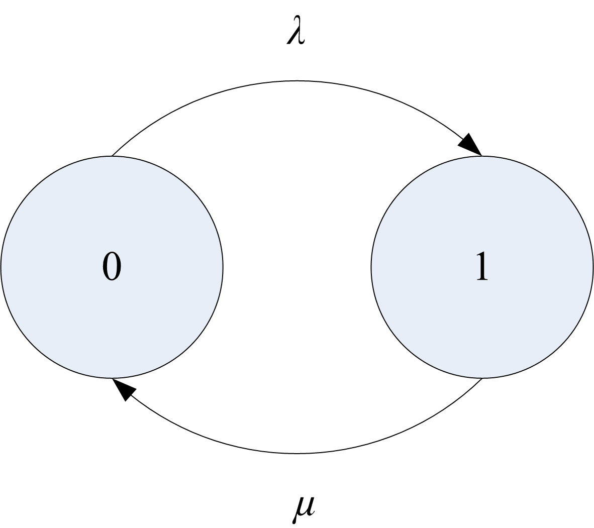
Figure C.4: Two state rate transition diagram
The rate of transition into state 0 can be thought of as the rate that probability flows from state 1 to state 0 times the chance of being in state 1, i.e. \(\mu P_1\). The rate of transition out of state 0 can be thought of as the rate from state 0 to state 1 times the chance of being in state 0, i.e. \(\lambda P_0\). Using these ideas yields:
| State | rate in | = | rate out |
|---|---|---|---|
| 0 | \(\mu\) \(P_1\) | = | \(\lambda\) \(P_0\) |
| 1 | \(\lambda\) \(P_0\) | = | \(\mu\) \(P_1\) |
Notice that these are identical equations, but with the fact that \(P_0 + P_1 = 1\), we will have two equations and two unknowns (\(P_0 , P_1\)). Thus, the equations can be easily solved to yield the same results as in Equation (C.3) and Equation (C.4). Sets of equations derived in this manner are called steady state equations.
Now, more general situations can be examined. Consider a general queueing system with some given number of servers. An arrival to the system represents an increase in the number of customers and a departure from the system represents a decrease in the number of customers in the system.
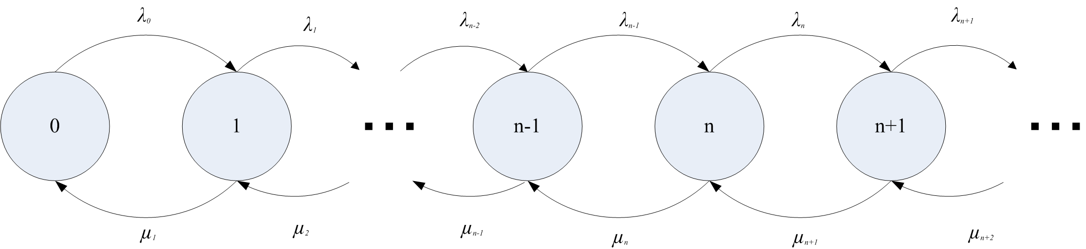
Figure C.5: General rate transition diagram for any number of states
Figure C.5 illustrates a general state transition diagram for this system. Let \(N\) be the number of customers in the system in steady state and define:
\[P_n = P\lbrace N=n\rbrace = \lim_{t \to \infty}P\lbrace N(t) = n\rbrace\]
as the steady state probability that there are \(n\) customers in the system. Let \(\lambda_n\) be the mean arrival rate of customers entering the system when there are \(n\) customers in the system, \(\lambda_n \geq 0\). Let \(\mu_n\) be the mean service rate for the overall system when there are \(n\) customers in the system. This is the rate, at which customers depart when there are \(n\) customers in the system. In this situation, the number of customers may be infinite, i.e. \(N \in \lbrace 0,1,2,\ldots\rbrace\). The steady state equations for this situation are as follows:
| State | rate in | = | rate out |
|---|---|---|---|
| 0 | \(\mu_1 P_1\) | = | \(\lambda_0 P_0\) |
| 1 | \(\lambda_0 P_0 + \mu_2 P_2\) | = | \(\mu_1 P_1 + \lambda_1 P_1\) |
| 2 | \(\lambda_1 P_1 + \mu_3 P_3\) | = | \(\mu_2 P_2 + \lambda_2 P_2\) |
| \(\vdots\) | \(\vdots\) | \(\vdots\) | \(\vdots\) |
| \(n\) | \(\lambda_{n-1} P_{n-1} + \mu_{n+1} P_{n+1}\) | = | \(\mu_n P_n + \lambda_n P_n\) |
These equations can be solved recursively starting with state 0. This yields:
\[ P_1 = \frac{\lambda_0}{\mu_1} P_0 \] \[ P_2 = \frac{\lambda_1 \lambda_0}{\mu_2 \mu_1} P_0 \]
\[ \vdots \] \[ P_n = \frac{\lambda_{n-1} \lambda_{n-2}\cdots \lambda_0}{\mu_n \mu_{n-1} \cdots \mu_1} P_0 = \prod_{j+1}^{n-1}\biggl(\frac{\lambda_j}{\mu_{j+1}}\biggr) P_0 \]
for \(n = 1,2,3, \ldots\). Provided that \(\sum_{n=0}^{\infty} P_n = 1\), \(P_0\) can be computed as:
\[P_0 = \Biggl[\sum_{n=0}^{\infty} \prod_{j=0}^{n-1}\biggl(\dfrac{\lambda_j}{\mu_{j+1}}\biggr)\Biggr]^{-1}\]
Therefore, for any given set of \(\lambda_n\) and \(\mu_n\), one can compute \(P_n\). The \(P_n\) represent the steady state probabilities of having \(n\) customers in the system. Because \(P_n\) is a probability distribution, the expected value of this distribution can be computed. What is the expected value for the \(P_n\) distribution? The expected number of customers in the system in steady state. This is \(L\). The expected number of customers in the system and the queue are given by:
\[\begin{aligned} L & = \sum_{n=0}^{\infty} nP_n \\ L_q & = \sum_{n=c}^{\infty} (n-c)P_n\end{aligned}\]
where \(c\) is the number of servers.
There is one additional formula that is needed before Little’s formula can be applied with other known relationships. For certain systems, e.g. finite system size, not all customers that arrive will enter the queue. Little’s formula is true for the customers that enter the system. Thus, the effective arrival rate must be defined. The effective arrival rate is the mean rate of arrivals that actually enter the system. This is given by computing the expected arrival rate across the states. For infinite system size, we have:
\[\lambda_e = \sum_{n=0}^{\infty} \lambda_n P_n\]
For finite system size, \(k\), we have:
\[\lambda_e = \sum_{n=0}^{k-1} \lambda_n P_n\]
since \(\lambda_n = 0\) for \(n \geq k\). This is because nobody can enter when the system is full. All these relationships yield:
\[\begin{aligned} L & = \lambda_e W \\ L_q & = \lambda_e W_q\\ B & = \frac{\lambda_e}{\mu} \\ \rho & = \frac{\lambda_e}{c\mu}\\ L & = L_q + B \\ W & = W_q + \frac{1}{\mu}\end{aligned}\]
Section C.4 presents the results of applying the general solution for \(P_n\) to different queueing system configurations. Table C.1 presents specific results for the M/M/c queuing system for \(c = 1,2,3\). Using these results and those in Section C.4, the analysis of a variety of different queueing situations is possible.
| \(c\) | \(P_0\) | \(L_q\) |
|---|---|---|
| 1 | \(1 - \rho\) | \(\dfrac{\rho^2}{1 - \rho}\) |
| 2 | \(\dfrac{1 - \rho}{1 + \rho}\) | \(\dfrac{2 \rho^3}{1 - \rho^2}\) |
| 3 | \(\dfrac{2(1 - \rho)}{2 + 4 \rho + 3 \rho^2}\) | \(\dfrac{9 \rho^4}{2 + 2 \rho - \rho^2 - 3 \rho^3}\) |
This section has only scratched the surface of queueing theory. A vast amount of literature is available on queueing theory and its application. You should examine (Gross and Harris 1998), (Cooper 1990), and (Kleinrock 1975) for a more in depth theoretical development of the topic. There are also a number of free on-line resources available on the topic. The interested reader should search on “Queueing Theory Books On Line.” The next section presents some simple examples to illustrate the use of the formulas.