7.6 Exercises
Exercise 7.1 Suppose a service facility consists of two stations in series (tandem), each with its own FIFO queue. Each station consists of a queue and a single server. A customer completing service at station 1 proceeds to station 2, while a customer completing service at station 2 leaves the facility. Assume that the inter-arrival times of customers to station 1 are IID exponential random variables with a mean of 1 minute. Service times of customers at station 1 are exponential random variables with a mean of 0.7 minute, and at station 2 are exponential random variables with mean 0.9 minute. Assume that the travel time between the two stations must be modeled. The travel time is distributed according to a triangular distribution with parameters (1, 2, 4) minutes.
Model the system assuming that the worker from the first station moves the parts to the second station. The movement of the part should be given priority if there is another part waiting to be processed at the first station.
Model the system with a new worker (resource) to move the parts between the stations.
From your models, estimate the total system time for the parts, the utilization of the workers, and the average number of parts waiting for the workers. Run the simulation for exactly 20000 minutes with a warm up period of 5000 minutes.
Model the system and estimate the total system time for the parts, the utilization of the workers, and the average number of parts waiting for the fork truck. Run the simulation for exactly 20000 minutes with a warm up period of 5000 minutes.
Instead of immediately moving the part, the fork truck waits until a batch of 5 parts has been produced at the first station. When this occurs, the fork truck is called to move the batch of parts to the second station. The parts are still processed individually at the second station. Redo the analysis of part (a) for this situation.
Exercise 7.8 Reconsider Exercise 7.4. The distances between the four stations (in feet) are given in the following table. After the parts finish the processing at the last station of their sequence they are transported to an exit station, where they begin their shipping process.
| Station | A | B | C | D | Exit | |
| A | – | 50 | 60 | 80 | 90 | |
| B | 55 | – | 25 | 55 | 75 | |
| C | 60 | 20 | – | 70 | 30 | |
| D | 80 | 60 | 65 | – | 35 | |
| Exit | 100 | 80 | 35 | 40 | – |
There are 2 fork trucks in the system. The velocity of the fork trucks varies within the facility due to various random congestion effects. Assume that the fork truck’s velocity between the stations is triangularly distributed with parameters (3, 4, 5) miles per hour. Simulate the system for 30000 minutes and discuss the potential bottlenecks in the system.
Exercise 7.9 Reconsider the Test and Repair example from Section 7.2.1 In this problem, the workers have a home base that they return to whenever there are no more waiting requests rather than idling at their last drop off point. The home base is located at the center of the shop. The distances from each station to the home base are given in as follows.
| Station | Diagnostics | Test 1 | Test 2 | Test 3 | Repair | Home base | |
| Diagnostics | – | 40 | 70 | 90 | 100 | 20 | |
| Test 1 | 43 | – | 10 | 60 | 80 | 20 | |
| Test 2 | 70 | 15 | – | 65 | 20 | 15 | |
| Test 3 | 90 | 80 | 60 | – | 25 | 15 | |
| Repair | 110 | 85 | 25 | 30 | – | 25 | |
| Home base | 20 | 20 | 15 | 15 | 25 | – |
Update the animation so that the total number of waiting requests for movement is animated by making it visible at the home base of the workers. Rerun the model using the same run parameters as the chapter example and report the average number of requests waiting for transport. Give an assessment of the risk associated with meeting the contract specifications based on this new design.
Exercise 7.10 Reconsider Exercise 6.12 with transporters to move the parts between the stations. The stations are arranged sequentially in a flow line with 25 meters between each station, with the distances provided as follows:
| Station | 1 | 2 | 3 | Exit | |
| 1 | – | 25 | 50 | 75 | |
| 2 | 25 | – | 25 | 50 | |
| 3 | 50 | 25 | – | 25 | |
| Exit | 75 | 50 | 25 | – |
Assume that there are two transporters available to move the parts between the stations. Whenever a part is required at a down stream station and a part is available for transport the transporter is requested. If no part is available, no request is made. If a part becomes available, and a part is need, then the transporter is requested. The velocity of the transporter is considered to be TRIA(22.86, 45.72, 52.5)in meters per minute. By using the run parameters of Exercise 6.12, estimate the effect of the transporters on the throughput of the system.
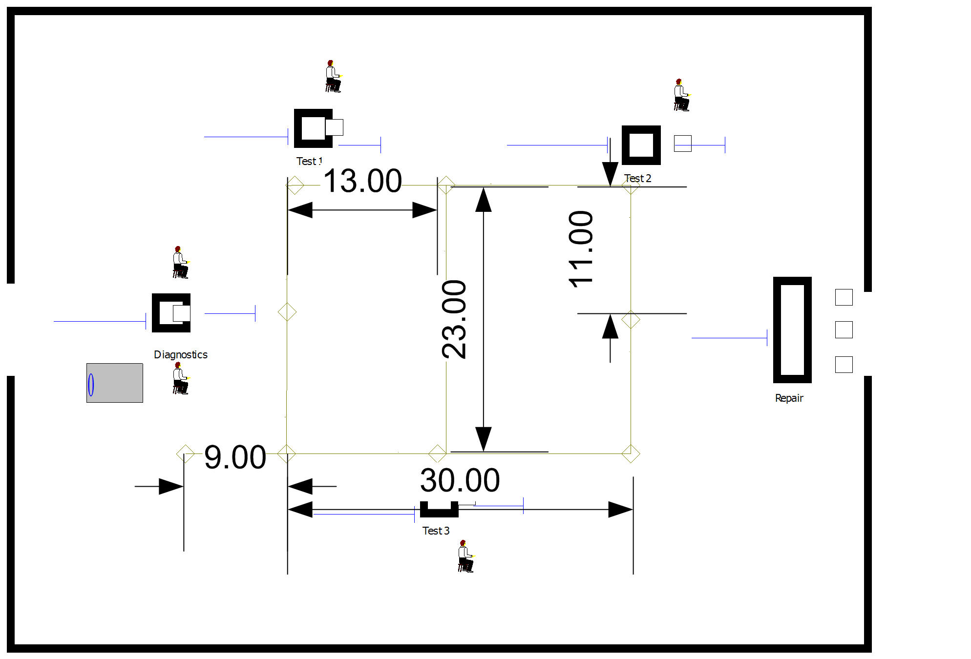
Figure 7.52: Proposed system layout
There is only 1 AGV in this system. It is 1 meter in length and moves at a velocity of 30 meters per minute. Its home base is at the dead end of the 9 meter spur. Since there will be only one AGV all links are bidirectional. The design associates the stations with the nearest intersection on the path network.
Simulate the system for 10 replications of 4160 hours. Estimate the chance that the contract specifications are met and the average system time of the jobs. In addition, assess the queuing for and the utilization of the AGV.
Consider the possibility of having a 2 AGV system. What changes to your design do you recommend? Be specific enough that you could simulate your design.
| Enter | Workstation | Paint | New Paint | Pack | Exit | |
|---|---|---|---|---|---|---|
| Enter | – | 325 | 445 | 445 | 565 | 815 |
| Workstation | – | 120 | 130 | 240 | 490 | |
| Paint | – | 250 | 120 | 370 | ||
| New Paint | – | 130 | 380 | |||
| Pack | – | 250 | ||||
| Exit | – |
The distances are symmetric. Both the drop-off and pickup points at a station are at the same physical location. Once the truck reaches the pickup/drop-off station, it requires a load/unload time of two minutes.
Analyze this system to determine any potential bottleneck operations. Report on the average flow times of the parts as a whole and individually. Also obtain statistics representing the average number of parts waiting for allocation of a transporter and the number of busy transporters. Run the model for 600,000 minutes with a 50,000 minute warm up period. Develop an animation for this system that illustrates the transport and queuing within the system.
Exercise 7.15 (This problem is based on an example on page 381 of (Pegden, Shannon, and Sadowski 1995). Used with permission). Reconsider Exercise 7.14 with the use of AGVs. There are now 3 AGVs that travel at a speed of 100 feet per minute to transport the parts within the system.
To avoid deadlock situations the guided path network has been designed for one way travel. In addition, to prevent an idle vehicle from blocking vehicles performing transports, a staging area (Intersection 12)has been placed on the guided path network. Whenever a vehicle completes a transport, a check should be made of the number of requests pending for the transporters. If there are no requests pending, the AGV should be sent to the staging area. If there are multiple vehicles idle, they should wait on Link 11. Link 15 is a spur from intersection 6 to intersection 11. The stations for the operation on the parts should be assigned to the intersections as shown in the figure. The links should all be divided into zones of 10 feet each. The initial position of the vehicles should be along Link 11. Each vehicle is 10 feet in length or 1 zone. The release at start form of zone control should be used.
The guided path network for the AGVs is given in Figure 7.53:
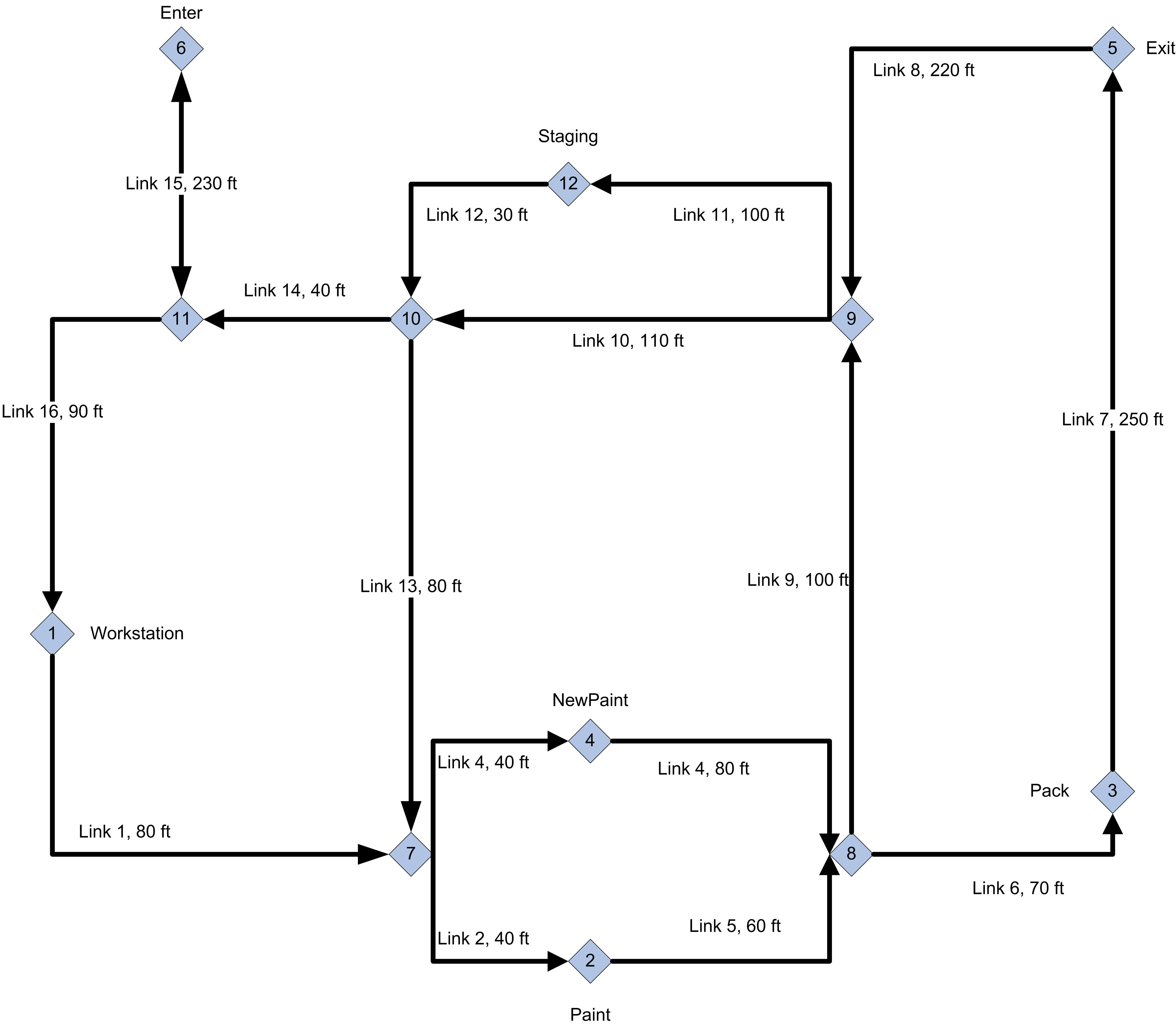
Figure 7.53: AGV system layout
Analyze this system to determine any potential bottleneck operations. Report on the average flow times of the parts as a whole and individually. Also obtain statistics representing the average number of parts waiting for allocation of a transporter and the number of busy transporters. Run the model for 600,000 minutes with a 50,000 minute warm up period. Develop an animation for this system that illustrates the transport and queuing within the system.
| Station | Production Rate | Tote Loading Time | Travel distance to next station |
|---|---|---|---|
| Machine 1 | 2 per minute | uniform(3,5) seconds | 40 meters |
| Machine 2 | 1 per minute | uniform(2,5) seconds | 28 meters |
| Machine 3 | 3 per minute | uniform(4,6) seconds | 55 meters |
The AGV moves from station to station in the sequence (Machine 1, Machine 2, Machine 3, store room). If there are totes waiting at the machine’s loading area, the AGV loads the totes up to its capacity. After the loading is completed, the AGV moves to the next station. If there are no totes waiting at the station, the AGV delays for 5 seconds, if any totes arrive during the delay they are loaded; otherwise, the AGV proceeds to the next station. After visiting the third machine’s station, the AGV proceeds to the store room. At the storeroom any totes that the AGV is carrying are dropped off. The AGV is designed to release all totes at once, which takes between 8 and 12 seconds uniformly distributed. After completing its visit to the store room, it proceeds to the first machine. The distance from the storeroom to the first station is 30 meters. The AGV travels at a velocity of 30 meters per minute. Simulate the performance of this system over a period of 10,000 minutes.
Estimate the average system time for a part. What is the average number of totes carried by the AGV? What is the average route time? That is, what is the average time that it takes for the AGV to complete one circuit of its route?
Suppose the sizing of the loading area for the totes is of interest. What is the required size of the loading area (in terms of the number of totes) such that the probability that all totes can wait is virtually 100%.