B.1 Random Variables and Probability Distributions
This section discusses some concepts in probability and statistics that are especially relevant to simulation. These will serve you well as you model randomness in the inputs of your simulation models. When an input process for a simulation is stochastic, you must develop a probabilistic model to characterize the process’s behavior over time. Suppose that you are modeling the service times in the pharmacy example. Let \(X_i\) be a random variable that represents the service time of the \(i^{th}\) customer. As shown in Figure B.1, a random variable is a function that assigns a real number to each outcome, \(s\), in a random process that has a set of possible outcomes, \(S\).
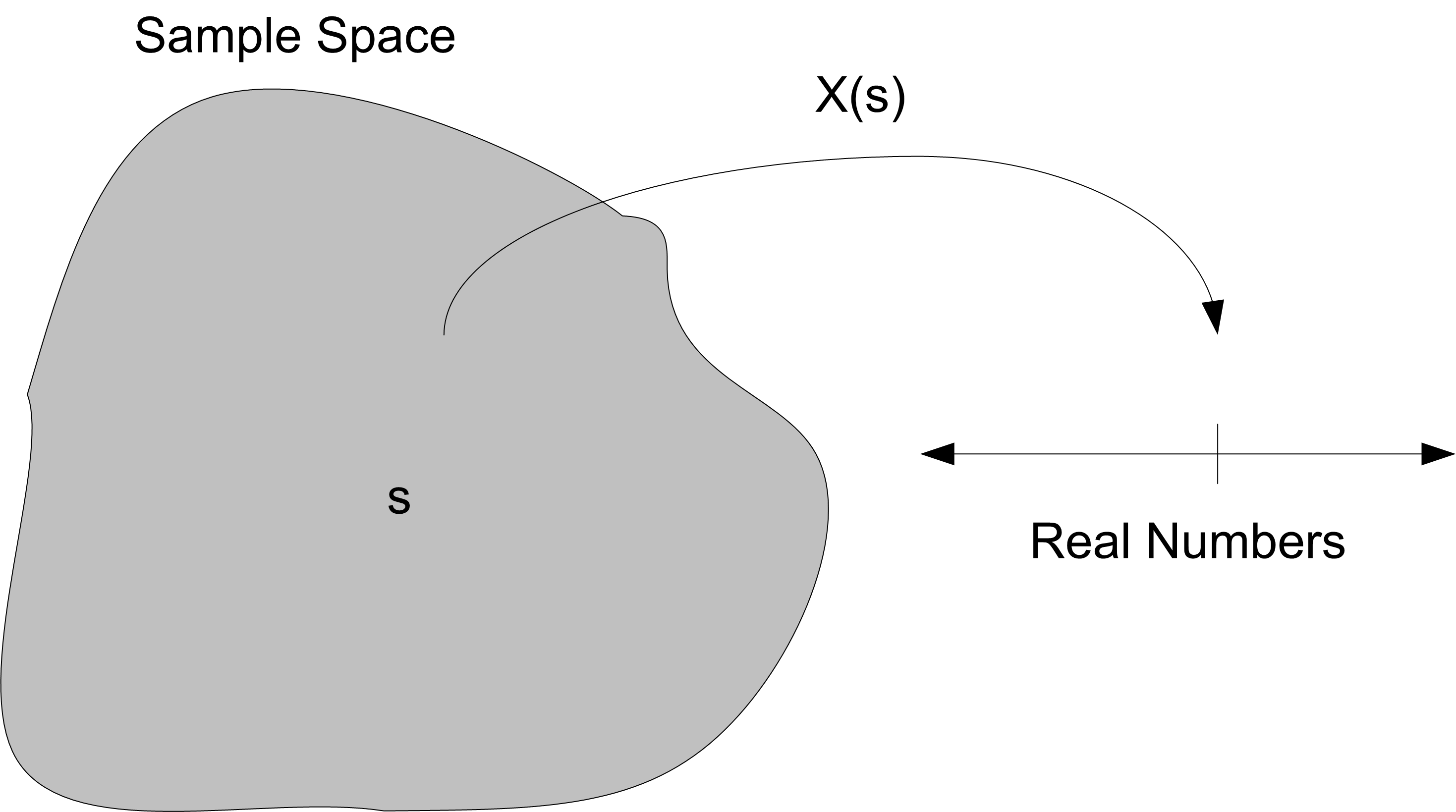
Figure B.1: Random Variables Map Outcomes to Real Numbers
In this case, the process is the service times of the customers and the outcomes are the possible values that the service times can take on, i.e. the range of possible values for the service times.
The determination of the range of the random variable is part of the modeling process. For example, if the range of the service time random variable is the set of all possible positive real numbers, i.e. \(X_i \in \Re^+\) or in other words, \(X_i \geq 0\), then the service time should be modeled as a continuous random variable.
Suppose instead that the service time can only take on one of five discrete values 2, 5, 7, 8, 10, then the service time random variable should be modeled as a discrete random variable. Thus, the first decision in modeling a stochastic input process is to appropriately define a random variable and its possible range of values.
The next decision is to characterize the probability distribution for the random variable. As indicated in Figure B.2, a probability distribution for a random variable is a function that maps from the range of the random variable to a real number, \(p \in [0,1]\). The value of \(p\) should be interpreted as the probability associated with the event represented by the random variable.
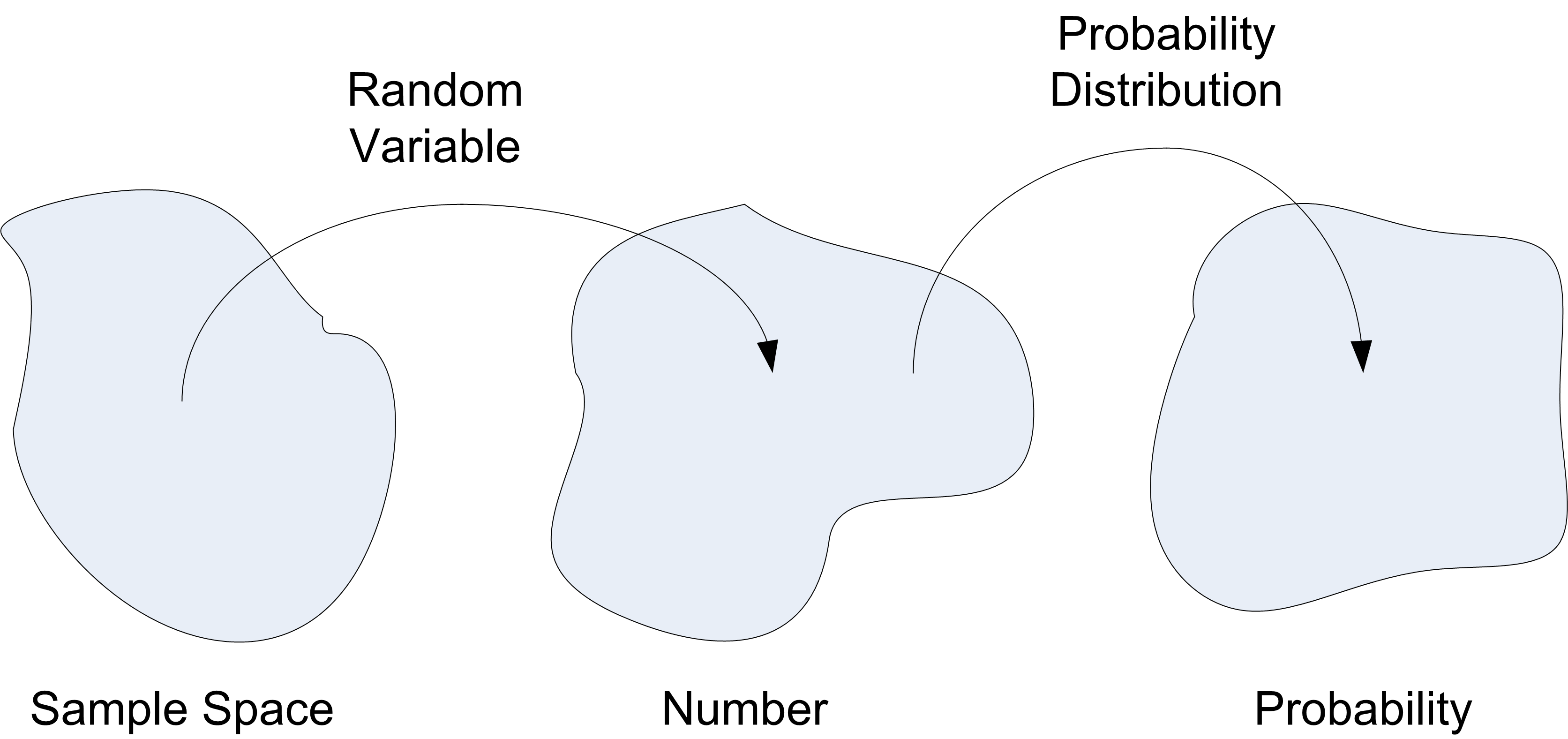
Figure B.2: robability Distributions Map Random Variables to Probabilities
For a discrete random variable, \(X\), with possible values \(x_1, x_2, \ldots x_n\) (n may be infinite), the function, \(f(x)\) that assigned probabilities to each possible value of the random variable is called the probability mass function (PMF) and is denoted:
\[f(x_i) = P(X = x_i)\]
where \(f(x_i) \geq 0\) for all \(x_i\) and \(\sum\nolimits_{i = 1}^{n} f(x_i) = 1\). The probability mass function describes the probability value associated with each discrete value of the random variable.
For a continuous random variable, \(X\), the mapping from real numbers to probability values is governed by a probability density function, \(f(x)\) and has the properties:
\(f(x) \geq 0\)
\(\int_{-\infty}^\infty f(x)dx = 1\) (The area must sum to 1.)
\(P(a \leq x \leq b) = \int_a^b f(x)dx\) (The area under f(x) between a and b.)
The probability density function (PDF) describes the probability associated with a range of possible values for a continuous random variable.
A cumulative distribution function (CDF) for a discrete or continuous random variable can also be defined. For a discrete random variable, the cumulative distribution function is defined as
\[F(x) = P(X \leq x) = \sum_{x_i \leq x} f(x_i)\]
and satisfies, \(0 \leq F(x) \leq 1\), and for \(x \leq y\) then \(F(x) \leq F(y)\).
The cumulative distribution function of a continuous random variable is
\[F(x) = P(X \leq x) = \int_{-\infty}^x f(u) du \; \text{for} \; -\infty < x < \infty\]
Thus, when modeling the elements of a simulation model that have randomness, one must determine:
Whether or not the randomness is discrete or continuous
The form of the distribution function (i.e. the PMF or PDF)
To develop an understanding of the probability distribution for the random variable, it is useful to characterize various properties of the distribution such as the expected value and variance of the random variable.
The expected value of a discrete random variable \(X\), is denoted by \(E[X]\) and is defined as:
\[E[X] = \sum_x xf(x)\]
where the sum is defined through all possible values of \(x\). The variance of \(X\) is denoted by \(Var[X]\) and is defined as:
\[\begin{split} Var[X] & = E[(X - E[X])^2] \\ & = \sum_x (x - E[X])^2 f(x) \\ & = \sum_x x^2 f(x) - (E[X])^2 \\ & = E[X^2] - (E[X])^2 \end{split}\]
Suppose \(X\) is a continuous random variable with PDF, \(f(x)\), then the expected value of \(X\) is
\[E[X] = \int_{-\infty}^\infty xf(x) dx\]
and the variance of X is
\[Var[X] = \int_{-\infty}^\infty (x - E[X])^2 f(x)dx = \int_{-\infty}^\infty x^2 f(x)dx -(E[X])^2\]
which is equivalent to \(Var[X] = E[X^2] - (E[X])^2\) where
\[E[X^2] = \int_{-\infty}^\infty x^2 f(x)\]
Another parameter that is often useful is the coefficient of variation. The coefficient of variation is defined as:
\[c_v = \frac{\sqrt{Var[X]}}{E[X]}\]
The coefficient of variation measures the amount of variation relative to the mean value (provided that \(E\{X\} \neq 0\)).
To estimate \(E\{X\}\), the sample average, \(\bar{X}(n)\),
\[\bar{X}(n) = \frac{1}{n}\sum_{i=1}^{n}X_i\]
is often used. To estimate \(Var[X]\), assuming that the data are independent, the sample variance, \(S^{2}\),
\[S^{2}(n) = \frac{1}{n-1}\sum_{i=1}^{n}(X_i - \bar{X})^2\]
can be used. Thus, an estimator for the coefficient of variation is:
\[\hat{c}_v = \frac{s}{\bar{x}}\]
A number of other statistical quantities are also useful when trying to characterize the properties of a distribution:
skewness - Measures the asymmetry of the distribution about its mean.
kurtosis - Measures the degree of peakedness of the distribution
order statistics - Used when comparing the sample data to the theoretical distribution via P-P plots or Q-Q plots.
quantiles (1st quartile, median, 3rd quartile) - Summarizes the distribution of the data.
minimum, maximum, and range - Indicates the range of possible values
Skewness can be estimated by:
\[\hat{\gamma}_{1} = \frac{\frac{1}{n}\sum\nolimits_{i=1}^{n}\left(X_i - \bar{X}\right)^3}{\left[S^2\right]^{3/2}}\]
For a unimodal distribution, negative skew indicates that the tail on the left side of the PDF is longer or fatter than the right side. Positive skew indicates that the tail on the right side is longer or fatter than the left side. A value of skewness near zero indicates symmetry.
Kurtosis can be estimated by:
\[\hat{\gamma}_{2} = \frac{n-1}{(n-2)(n-3)}\left((n+1) g_{2} +6\right)\]
where, \(g_{2}\) is:
\[g_{2} = \frac{\frac{1}{n}\sum\nolimits_{i=1}^{n}\left(X_i - \bar{X}\right)^4}{\left(\frac{1}{n}\sum\nolimits_{i=1}^{n}\left(X_i - \bar{X}\right)^2\right)^2} -3\]
Order statistics are just a fancy name for the the sorted data. Let (\(x_1, x_2, \ldots x_n\)) represent a sample of data. If the data is sorted from smallest to largest, then the \(i^{th}\) ordered element can be denoted as,\(x_{(i)}\). For example, \(x_{(1)}\) is the smallest element, and \(x_{(n)}\) is the largest, so that (\(x_{(1)}, x_{(2)}, \ldots x_{(n)}\)) represents the ordered data and these values are called the order statistics. From the order statistics, a variety of other statistics can be computed:
minimum = \(x_{(1)}\)
maximum = \(x_{(n)}\)
range = \(x_{(n)} - x_{(1)}\)
The median, \(\tilde{x}\), is a measure of central tendency such that one-half of the data is above it and one-half of the data is below it. The median can be estimated as follows:
\[\tilde{x} = \begin{cases} x_{((n + 1)/2)} & n \text{ is odd}\\ \dfrac{x_{(n/2)} + x_{((n/2) + 1)}}{2} & n \text{ is even}\\ \end{cases}\]
For example, consider the following data:
\[x_{(1)} = 3, x_{(2)} = 5, x_{(3)} = 7, x_{(4)} = 7, x_{(5)} = 38\]
Because \(n = 5\), we have:
\[\dfrac{n + 1}{2} = \dfrac{5 + 1}{2} = 3\]
\[\tilde{x} = x_{(3)} = 7\]
Suppose we have the following data: \[x_{(1)} = 3, x_{(2)} = 5, x_{(3)} = 7, x_{(4)} = 7\]
Because \(n=4\), we have:
\[\begin{aligned} x_{(n/2)} & = x_{(2)}\\ x_{((n/2) + 1)} & = x_{(3)}\\ \tilde{x} & = \dfrac{x_{(2)} + x_{(3)}}{2} = \dfrac{5 + 7}{2} = 6\end{aligned}\]
The first quartile is the first 25% of the data and can be thought of as the ‘median’ of the first half of the data. Similarly, the third quartile is the first 75% of the data or the ‘median’ of the second half of the data. Different methods are used to estimate these quantities in various software packages; however, their interpretation is the same, summarizing the distribution of the data.
As noted in this section, a key decision in distribution modeling is whether the underlying random variable is discrete or continuous. The next section discusses how to model discrete distributions.