4.1 Enhancing the STEM Career Mixer Example
In Chapter 3, we discussed the implementation of an Arena model for the STEM Career Fair Mixer of Example 3.4. In this section, we are going to embellish the system to add a few modeling issues that will make the model a bit more realistic. This will also allow for the introduction of the following new Arena modules.
EXPRESSION
ROUTE
STATION
STORAGE
STORE
UNSTORE
We will also re-examine how the CREATE module works and see how to collect additional performance metrics. Finally, we will learn how to control the underlying random number streams used when generating random variables within Arena.
The following issues will be addressed in the new model.
In reality, those students that wander around before deciding to visit the recruiters actually visit the conversation area associated with the mixer. The organizer of the event has asked alumni to volunteer to be available within the conversation area to chat with students and discuss their career development. After all, it is a mixer. The organizer of the mixer would like to plan for the size of the conversation area.
The STEM Fair is scheduled for 6 hours; however, currently, the simulation simply ends “abruptly” at 6 hours. How should we handle those students that are attending the mixer when the mixer ends? In this section, we will model a more realistic approach to ending the mixer and handling the students in progress.
After discussing with the STEM Fair organizer, the following additional facts were discovered. Generally, near the end of the scheduled mixer time, an announcement is made to everyone in the facility through the public address (PA) system that the mixer will be ending soon. For the purposes of this modeling enhancement, we can assume that the announcement goes out 15 minutes before the end of the mixer. At that time, we can assume the following:
The doors to the mixture are closed to new arrivals. In other words, a closed sign goes up so that no new students are admitted to the mixer.
Any students that were chatting within the conversation area finish up their conversations and then head for the exit, without visiting the recruiting stations.
Any student walking to the name tag area, the conversation area or to the recruiting area proceed to the exit.
Any students already at the recruiting stations, either in line waiting, or talking with the recruiter are allowed to finish up their visit and then depart the mixer.
Based on additional observations and discussion with the STEM mixer organizer, the following changes can be assumed:
Because the distances between the stations in the hall are now important an enhanced drawing of the system has been made that better illustrates the standard layout that has been used in the past for the mixer. The distances shown in the drawing are rough estimates.
New data suggest that 60% of the arriving students do not visit the conversation area, but instead go directly to the recruiting area to pick one of the two recruiting stations to visit, with equal probability.
The remaining 40% of students will first visit the conversation area. The time spent within the conversation area is a little less than previously noted to exclude the time spent walking. The conversation time is triangularly distribution with a minimum of 10 minutes, a most likely value of 15 minutes, and a maximum value of 30 minutes. After having their conversations, 90% of the students decide to visit one of the two recruiting stations. The other 10% are too tired or timid and decide to leave.
The speed of people walking can vary greatly, but prior data suggests that for short distances within and around buildings, people walk between 1 mile per hour and 3 miles per hour, with a most likely time of 2 miles per hour, triangularly distributed.
After further conversations with students who have attended past mixers, it was discovered that there really isn’t a preference for visiting one of the recruiters first. Instead, after arriving to the recruiting area, students decide to visit the recruiter that has the least number of people (waiting and interacting with the recruiters). If both recruiter locations have the same total number of students, then the students show no preference between the two recruiters. After visiting the first recruiter, if they have already spent more than 45 minutes at the STEM fair, they decide to depart; otherwise, they visit the recruiter that they have not yet visited. After visiting both, they depart.
Because of these changes to the modeling assumptions, the STEM organizer would like to better understand the following aspects of potential system performance.
When the PA announcement occurs, how many students on average are:
In the conversation area
Attending the MalWart recruiting station
Attending the JHBunt recruiting station
How long after the 6-hour scheduled time does the mixer actually end? That is, since all students are permitted to finish up what they are currently doing when the PA announcement occurs, how long does it take for the hall to be completely empty?
How many students, on average, are in the conversation area?
The probability that a student departs because they have already spent more than 45 minutes at the mixer after visiting their first recruiting station.
For students that do not visit the conversation area, what is the probability that their system time is less than 30 minutes?
Given this new description there are two major modeling issues that need to be addressed:
how to close the mixer and
modeling and visualizing the walking.
4.1.1 Turning Off a CREATE Module
In order to better model the closing of the mixer, we need to understand how to turn off a CREATE module. As shown in Figure 4.1, the CREATE module has a field labeled “Max Arrivals.” For every CREATE module there is an internal variable that counts how many creation events have occurred. During the simulation, this variable is automatically compared to the current value of the field labeled “Max Arrivals” and if the internal variable becomes greater than or equal to the current value of the field “Max Arrivals” then the CREATE module stops its creation process. For example, suppose that the value of Max Arrivals was 10. Then, only 10 creation events will occur.
By using a variable, say vMaxNumArrivals, the user can specify how many arrivals there should be. When you want to turn off the CREATE module just set the value of vMaxNumArrivals to 0. So, to close the door for the STEM mixer we will use another CREATE module that will cause the value of vMaxNumArrivals to be set to zero, at time 345 minutes (i.e. 15 minutes before the end of the mixer). This will also facilitate the collection of the additional performance measures.
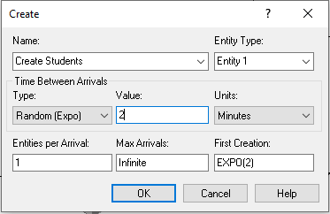
Figure 4.1: Example CREATE module
4.1.2 Modeling Walking Time
To model the walking within the mixer, we need to translate the distance travelled into time. Since we are told the typical velocity for walking within a building for a person, we can randomly generate the velocity associated with a walking trip. Then, if we know the distance to walk, we can determine the time via the following relationship, where \(v\) is the speed (velocity), \(d\) is the distance, and \(t\) is the time.
\[v = \frac{d}{t}\]
Thus, we can randomly generate the value of \(v\), and use the relationship to determine the time taken.
\[t = \frac{d}{v}\]
We know that the speed of people walking is triangularly distributed with a minimum of 1 mile per hour, a mode of 2 miles per hour, and a maximum of 3 miles per hour. This translates into a minimum of 88 feet per minute, a mode of 176 feet per minute, and a maximum of 264 feet per minute. Thus, we represent the speed as a random variable, Speed ~ TRIA(88, 176, 264) feet per minute and if we know the distance to travel, we can compute the time.
We have the following distances between the major locations of the system:
Entrance to Name Tags, 20 feet
Name Tags to Conversation Area, 30 feet
Name Tags to Recruiting Area (either JHBunt or MalMart), 80 feet
Name Tags to Exit, 140 feet
Conversation Area to Recruiting Area (either JHBunt or MalMart), 50 feet
Conversation Area to Exit, 110 feet
Recruiting Area (either JHBunt or MalMart) to Exit, 60 feet
For simplicity, we assume that the distance between the JHBunt and MalWart recruiting locations within the recruiting area can be ignored.
4.1.3 Using Expressions within an Arena Model
Within Arena mathematical expressions may be formed using combinations of integers, constants, attributes, variables, or random distributions. Conditional statements may also be used. Conditional expressions are evaluated as numerical expressions; a true condition is assigned a value of 1, and a false condition is assigned a value of 0. We have already used many expressions within the example models. Suppose we have some distribution (e.g. walking speed distribution) that we need to use in many places within the model. That is, we will need to enter the mathematical expression in many different fields within different modules within the model. Now suppose, after about a month of using the model, we decide that the expression needs to be updated because of some new data. Since the mathematical expression is used throughout the model, we need to find it everywhere that it is used. Of course, we could use the search and find capability associated with the Arena environment to make the edits; however, a much better approach is to use the EXPRESSION module found on the Advanced Process panel.
The EXPRESSION module permits the definition of a named expression. Then, the name of the expression can be used throughout the model, similar to how variables and attributes are used. The EXPRESSION module defines expressions and their associated values. An expression can contain any Arena-supported expression logic, including real values, Arena distributions, Arena or user-defined system variables, and combinations of these. Expressions can be single elements or one- or two-dimensional arrays. By defining and naming an expression, you can use that name throughout your model. Then, if there is an update of the expression, you need only edit the expression within the EXPRESSION module to change it everywhere that it is used in the model. Expressions are extremely useful, especially arrayed expressions. We will use an expression defined within the EXPRESSION module to represent the speed distribution within the new implementation of the model. As a naming convention, I append the letter “e” to the beginning of any of my expressions. For example, we will use the name “eWalkingSpeedRV” to represent the walking speed within the new implementation. By appending the letter “e” to the name of your expressions, you will know that it is a defined expression when you see it used within various modules.
4.1.4 Introducing the STATION, ROUTE, STORAGE, and SET Modules
Because the model stakeholders desire improved animation, we will also need to introduce some new Arena constructs: STATION, ROUTE, and STORAGE.
- STATION
The STATION module represents a named location to which entities can be transferred. Initially, one can think of stations as the label part of the Go To – Label construct found in standard programming languages; however, stations are more powerful than a simple label. Stations can be placed in sets and held within sequences. Stations are also necessary for mapping model logic transfers to a physical (spatial) representation of the world.
- ROUTE
The ROUTE module causes an entering entity to be transferred to a station with a possible time delay that accompanies the transfer. The entity leaves the route module and after the specified time delay reappears in the model at the specified station.
The STATION module is found on the Advanced Transfer panel. See Figure 4.2 for the edit by dialog view of the STATION module. For our current purposes, we can think of a STATION module as a fancy label. A STATION denotes a location within the model to and from which entity instances can be transferred. Stations work very much like labels; however, special entity transfer modules are needed to send the entities to and from stations. Those modules are found on the Advanced Transfer panel, one of which is the ROUTE module, as shown in Figure 4.3. For our current purposes, a ROUTE module can be thought of as a Goto Label module, where we specify a station as the destination rather than a named label. ROUTE modules allow for the specification of a time delay associated with the transfer from the current location to the destination. The nice thing about this is that there are convenient animation constructs available for showing the entities as they experience the transfer delay. We will use this capability to show the people walking between the areas within the STEM mixer. The other modules associated with the Advanced Transfer panel will be discussed in Chapter 7.
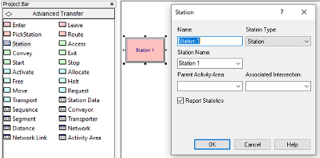
Figure 4.2: The STATION module
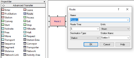
Figure 4.3: The ROUTE module
Finally, we will use the STORAGE module found on the Advanced Process panel to model the conversation areas associated with the STEM mixer. Figure 4.4 shows the STORAGE module as a data definition module on the Advanced Process panel. The STORAGE module is also a named location within the model. The STORAGE module simply creates and defines a storage that can be used within the model. The primary purpose of a storage is for animation; however, every storage has a special variable accessed through the function, NSTO(Storage Name), that returns the current number of entities associated with the storage. To place an entity in a storage, we use the STORE module and to take an entity out of storage, we use the UNSTORE module. The STORE and UNSTORE modules are also found on the Advanced Process Panel as illustrated in Figures 4.5 and 4.6. The STORE module automatically increments the number of entities in the associated storage by one and the UNSTORE module automatically decrements the number of entities in the associated storage by one. Thus, the variable, NSTO(Storage Name) can be used to collect statistics on the number of entities associated with the storage at any time. The nice thing about storages is that animated storages can be associated with the storage in order to display the entities currently in the storage during the animation. This capability could be use to show the students that are in the conversation area. In fact, a storage can be useful in animating the time that an entity is in the time delayed state.
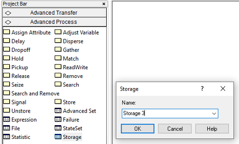
Figure 4.4: The STORAGE module
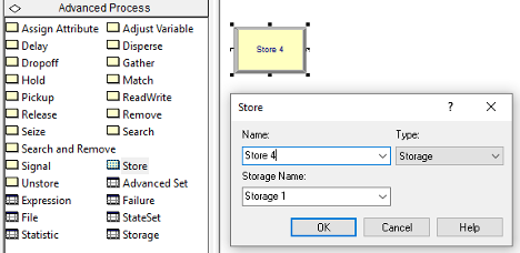
Figure 4.5: The STORE module
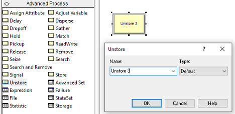
Figure 4.6: The UNSTORE module
The last new modeling construct that we will use within the implementation of the enhanced STEM Career Fair Mixer model is that of sets. Sets represent a set of similar elements held in an indexed list. Sets are an incredibly useful construct for implementing many useful modeling situations, especially the random selection of elements from the list. We will demonstrate the use of set by introducing tally sets (sets that hold tally statistics) and a station set (a set that holds a list of station). In the case of the station set, we will randomly select a station from the set and then send an entity to the station.
4.1.5 Controlling Randomness by Specifying Stream Numbers
Random number generators in computer simulation languages come with a default set of streams that divide a sequence of random numbers into independent sets (or sequences). The streams are only independent if you do not use up all the random numbers within the subsequence. These streams allow the randomness associated with a simulation to be controlled. During the simulation, you can associate a specific stream with specific random processes in the model. This has the advantage of allowing you to check if the random numbers are causing significant differences in the outputs. In addition, this allows the random numbers used across alternative simulations to be better synchronized.
Now a common question using simulation languages such as Arena can be answered. That is, “If the simulation is using random numbers, why to I get the same results each time I run my program?” The corollary to this question is, “If I want to get different random results each time I run my program, how do I do it?” The answer to the first question is that the underlying random number generator is starting with the same seed each time you run your program. Thus, your program will use the same pseudo random numbers today as it did yesterday and the day before, etc. The answer to the corollary question is that you must tell the random number generator to use a different seed (or alternatively a different stream) if you want different invocations of the program to produce different results. The latter is not necessarily a desirable goal. For example, when developing your simulation programs, it is desirable to have repeatable results so that you can know that your program is working correctly.
Since a random number stream is a sub-sequence of pseudo-random numbers that start at particular place with a larger sequence of pseudo-random numbers, it is useful to have a starting point for the sequence. The starting point of a sequence of pseudo-random numbers is called the seed. A seed allows us to pick a particular stream. Having multiple streams is useful to assign different streams to different sources of randomness within a model. This facilitates the control of the use of pseudo-random numbers when performing experiments. Every distribution in Arena has an extra optional parameter for the stream. For example, EXPO(mean, stream#), LOGN(mean, sd, stream#), DISC( cp1, v1, cp2, v2, .…, 1.0, vn, stream#), where stream# is some integer representing the stream you want to use for that distribution. Arena associates an integer number, 1, 2, 3, etc. with the seed associated with a particular random number stream. For all intents and purposes, we can assume that each stream produces independent random numbers.
To specify the stream in the CREATE module, use the "Expression" option for the type and then specify the distribution, e.g. EXPO(mean, 2). Use the expression option to specify the exact required expression. To control the stream associated with a DECIDE, use the DISC() function to assign an attribute, and then use a DECIDE module to check that attribute. For example:
// 40% chance for path 1, 60% chance for path 2, using stream 9
ASSIGN: myFlag = DISC(0.4, 1, 1.0, 2, 9)
DECIDE: If myFlag == 1,
   go to path 1
Else
   goto path 2
To prepare the STEM Mixer model for better control of the underlying randomness due to random number generation, the following stream assignments should be made.
Arrival process, stream 1
Name tag activity, stream 2
Choice to visit conversation area, stream 3
Choice between conversation areas, stream 4
Conversation time, stream 5
Deciding to visit recruiters after visiting conversation area, stream 6
Choice between MalMart and JHBunt, stream 7
MalMart interaction time, stream 8
JHBunt interaction time, stream 9
Walking speed, stream 10
Using streams to control the randomness will allow us to better implement a variance reduction technique called common random numbers when we make comparisons between system configurations. This will be discussed in Section 4.4.
Further details about how to generate random numbers and random variates are provided in Appendix A. The next section presents the pseudo-code for the revised STEM Mixer example.
4.1.6 Pseudo-code for the Revised STEM Mixer Example
Now we are ready to update the pseudo-code from Chapter 3 to address the previously discussed enhancements. The first thing to do is to define in the pseudo-code the modeling constructs that we will utilize. For this situation, we will define six new variables. The variable vClosed will be used to indicate that the mixer is closed. Then, we will have two new variables to keep track of how many students are visiting the MalWart and JHBunt recruiters, vNumAtMalWart and vNumAtJHBunt. Finally, we have three variables relate to the closing of the mixer: vMaxNumArrivals (to shut off the CREATE module), vWarningTime (to represent the time interval to the end of the mixer) and vMixerTimeLength (to represent the total time available for the mixer). These variables are defined in the following pseudo-code.
// Model Definition Pseudo-Code
ATTRIBUTES:
myType // represents the type of the student (1= recruiters first, 2 =
conversation first, 3 = timid).
myArrivalTime // the time that the student arrived to the mixer
myFirstRecruiter // the recruiter visited first
myNumVisits // the number of recruiters visited

VARIABLES:
vNumInSys // represents the number of students attending the mixer at any time t
vClosed = 0// represents that the STEM fair has closed its doors, 1 = closed, 0 = open
vNumAtJHBunt // number of students visiting JHBunt recruiters
vNumAtMalWart // number of students visiting MalWart recruiters
vMaxNumArrivals = 10000// used to control creation of students
vWarningTime = 15 // minutes, used to control when to close the STEM Mixer
vMixerTimeLength = 360 minutes

EXPRESSIONS:
eDoorClosingTime = vMixerTimeLength - vWarningTime
eWalkingSpeedRV = TRIA(88, 176, 264, 10)
eEntranceToNameTagsTimeRV = 20.0/eWalkingSpeedRV
eNameTagsToConverseAreaTimeRV = 30.0/eWalkingSpeedRV
eNameTagsToRecruitingAreaTimeRV = 80.0/eWalkingSpeedRV
eNameTagsToExitTimeRV = 140.0/eWalkingSpeedRV
eConverseAreaToRecruitingAreaTimeRV = 50.0/eWalkingSpeedRV
eConverseAreaToExitTimeRV = 110.0/eWalkingSpeedRV
eRecruitingAreaToExitTimeRV = 60.0/eWalkingSpeedRV

RESOURCES:
rMalWartRecruiters, 2 // the MalWart recruiters with capacity 2
rJHBuntRecruiters, 3 // the JHBunt recruiters with capacity 3

STORAGES:
stoConversationArea //use to show students in the conversation area

STATIONS:
staEntrance // the entrance to the mixer
staNameTag // the location to get name tags
staConverseArea // the area for holding conversations
staRecruitingArea // the area for visiting recruiters
staJHBunt // the JHBunt recruiting location
staMalWart // the MalMart recruiting location
staExit // the location to exit the mixer

SETS:
RecruiterStationSet (staJHBunt, staMarWart) // hold stations for picking between stations
SystemTimeSet(Type1SysTime, Type2SysTime, Type3SysTime) // to more easily collect statistics
In addition to variables, we have defined nine expressions, eight of which are related to the walking and time taken for movement between locations. A STORAGE has been defined to track the number of students in the conversation area and seven stations have been defined to represent locations. Finally, two sets are defined. The RecruiterStationSet holds the stations representing the JHBunt recruiting location and the MalWart recruiting location. The SystemTimeSet is a tally set that holds the tally statistical variables for collecting statistics by type of student. Now, we are ready to represent the model logic.
// Creating the Students
CREATE vMaxNumArrivals of students every EXPO(2,1) minutes with the
first arriving at time EXPO(2,1)
STATION staEntrance
BEGIN ASSIGN
   myArrivalTime = TNOW
   vNumInSys = vNumInSys + 1
END ASSIGN
ROUTE to staNameTag, time = eEntranceToNameTagsTimeRV
The logic for creating the students for the mixer is very similar to what was done in Chapter 3. The changes include having a variable, vMaxNumArrivals, to use to turn off the CREATE module and using a STATION to represent the entrance to the mixer. At the station, we assign the arrival time of the student for statistical collection and increment the number of students attending the mixer. Then, we use a ROUTE module to send the student to the name tag area using the time expression for modeling the walking from the entrance to the name tag area.
// Getting a Name Tag
STATION staNameTag
DECIDE IF vClosed == 1
   ROUTE to staExit, time = eNameTagsToExitTimeRV
END DECIDE
DELAY UNIF(15,45, 2) seconds to get name tag
ASSIGN myType = DISC(0.60, 1, 1.0, 2, 3) // 1 = recruiting only, 2 = conversation area
DECIDE If myType == 1 // recruiting station only student
   ROUTE to staRecruitingArea, time = eNameTagsToRecruitingAreaTimeRV
ELSE // myType = 2, conversation first student
   ROUTE to staConverseArea, time = eNameTagsToConverseAreaTimeRV
END DECIDE
The logic for getting a name tag has been updated to include sending students that were headed to the name tag area to the exit if the mixer closing warning occurred during their walk to the name tag area. Notice the specification of the stream number in the UNIF() distribution representing the time to get a name tag. Then, a DISC() distribution is use to determine the type of student and then the student is sent to the appropriate area via ROUTE modules. The pseudo-code for the conversation area, has the same check for closing during the walk to the location. Then, we see the use of the STORE and UNSTORE constructs to track how many students are in the conversation area during the delay for the conversation. Sending the students to the exit or to recruiting is used by assigning their type and then using a DECIDE to send them to the appropriate station.
// Visiting the Conversation Area
STATION staConverseArea
DECIDE IF vClosed == 1
   ROUTE to staExit, time = eConverseAreaToExitTimeRV
END DECIDE
STORE stoConversationArea
DELAY TRIA(10, 15, 30, 5) minutes for conversation
UNSTORE stoConversationArea
ASSIGN myType = DISC(0.9, 2, 1.0, 3, 6)
DECIDE If myType == 2 // recruiting station student
   ROUTE to staRecruitingArea, time = eConverseAreaToRecruitingAreaTimeRV
ELSE // myType = 3, timid student
   ROUTE to staExit, time = eConverseAreaToExitTimeRV
END DECIDE
After arriving to the recruiting area, we check if the mixer has closed and if so, send the student to the exit. Then, the logic checks the variables used to keep track of the number of students visiting JHBunt and MalWart are checked to determined which recruiter to visit. Notice the use of the DISC() distribution function in the case of ties. An attribute, myFirstRecruiter, is used to hold the choice, and then the appropriate station is selected from the recruiter station set based on the attribute. The use of a randomly assigned attribute to index into a set is a very useful pattern. Besides indexing into a set, this same idea can be used to randomly pick a value from an array or an expression.
// Visiting the Recruiting Area
STATION: staRecruitingArea
DECIDE IF vClosed == 1
   ROUTE to staExit, time = eRecruitingAreaToExitTimeRV
END DECIDE
DECIDE IF vNumAtJHBunt == vNumAtMalWart
   ASSIGN myFirstRecruiter = DISC(0.5, 1, 1.0, 2,7)
ELSE IF vNumAtJHBunt < vNumAtMalWart
   ASSIGN myFirstRecruiter = 1
ELSE
   ASSIGN myFirstRecruiter = 2
ENDIF
ROUTE with 0 delay, to RecruiterStationSet(myFirstRecruiter)
The pseudo-code for attending the MalWart or JHBunt recruiting stations is essentially the same. First we increment the number of students that are visiting and then process the students at the station.
// Attending MalWart
STATION: staMalWart
ASSIGN vNumAtMalWart = vNumAtMalWart + 1
SEIZE 1 MalWart recruiter
DELAY for EXPO(3,8) minutes for interaction
RELEASE 1 MalWart recruiter
ASSIGN vNumAtMalWart = vNumAtMalWart - 1
ASSIGN myNumVisits = myNumVisits + 1
DECIDE IF (myNumVisits == 1) AND (TNOW - myArrivalTime) > 45
   ASSIGN my45MinuteFlag = 1
   ROUTE to staExit, time = eRecruitingAreaToExitTimeRV
ELSE IF myNumVisits == 2
   ROUTE to staExit, time = eRecruitingAreaToExitTimeRV
ELSE
   ROUTE with 0 delay to staJHBunt
END DECIDE
The logic for determining which recruiter is visited next is interesting. Using an attribute, myNumVisits, allows us to determine if one or both recruiters have been visited. In the case of only one visit, we can determine whether or not the student has been at the mixer more than 45 minutes. If so, an attribute is used as an indicator variable to denote this event for later statistical processing. If both stations have been visited, then the student exits the mixer. If only one recruiter has been visited, then the student is sent to the opposite recruiter.
// Attending JHBunt
STATION: staJHBunt
ASSIGN vNumAtJHBunt = vNumAtJHBunt + 1
SEIZE 1 JHBunt recruiter
DELAY for EXPO(6,9) minutes for interaction
RELEASE 1 JHBunt recruiter
ASSIGN vNumAtJHBunt = vNumAtJHBunt - 1
ASSIGN myNumVisits = myNumVisits + 1
DECIDE IF (myNumVisits == 1) AND (TNOW -- myArrivalTime) > 45
   ASSIGN my45MinuteFlag = 1
   ROUTE to staExit, time = eRecruitingAreaToExitTimeRV
ELSE IF myNumVisits == 2
   ROUTE to staExit, time = eRecruitingAreaToExitTimeRV
ELSE
   ROUTE with 0 delay to staMalWart
END DECIDE
The exit area is primarily used to collect statistics on departing students. There are three updates to note. First, we can collect statistics on the probability that the students that do not visit the conversation have a system time that is less than or equal to 30 minutes. We use an expression (mySysTime <= 30) to collect on a logical indicator of this event. Secondly, we used a tally set to record the system times by student type (myType). Lastly, we director record on the indicator attribute, my45MinuteFlag, to collect the probability that the student exited after visiting only one recruiter because they had already been at the mixer for more than 45 minutes.
// Exiting and Collecting Statistics
STATION: staExit
ASSIGN: vNumInSys = vNumInSys - 1
ASSIGN: mySysTime = TNOW -- myArrivalTime
DECIDE IF myType == 1 // no conversation students
   RECORD (mySysTime <= 30)
END DECIDE
RECORD mySysTime, as System Time regardless of type
RECORD mySystTime, using SystemTimeSet by myType
RECORD my45MinuteFlag
DISPOSE
Now we have to model the closing of the STEM Mixer. As previously mentioned, we can do this by creating a logical entity that is used to turn off the CREATE module governing the creation of the students. We create one entity at the door closing time and close the door by changing the global variable, vClosed. In addition, we collect observation based statistics via RECORD statement that records the values of the variables at this particular instance in time. These are observation based statistics, not time persistent, because we are observing the random value at a particular instance of time (not over time).
// Model Pseudo-Code Listing for Closing the Mixer
CREATE 1 entity, at time eDoorClosingTime
ASSIGN vMaxNumArrivals = 0
ASSIGN vClosed = 1
RECORD Expressions // observe variables at door closing time
   NSTO(stoConversationArea)
   vNumAtMalWart
   vNumAtJHBunt
   vNumInSys
END RECORD
DISPOSE
Now that all the pseudo-code is specified, implementing the model in Arena is very straight-forward. We implement these ideas in the next section.
4.1.7 Implementing the Revised STEM Mixer Model in Arena
To implement this model within Arena, we can follow the pseudo-code starting with the model definitions. Figure 4.7 and 4.8 show the revised attributes and variables for the Arena model. It is best practice to define your modeling constructs first before using them in the Arena flow chart area. This allows you to select the construct from drop-down boxes or from within the expression builder rather than directly typing in the construct. This reduces the number of typos and other syntax errors.
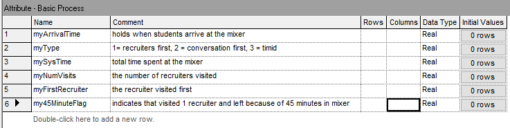
Figure 4.7: Defining the attributes for the revised STEM Mixer example
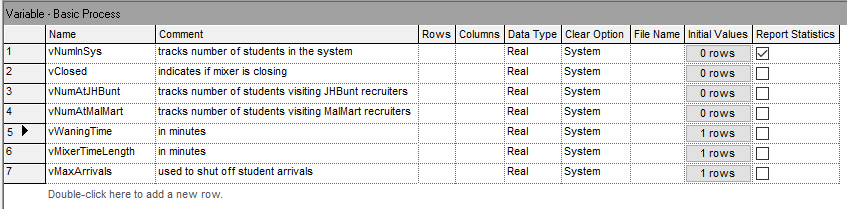
Figure 4.8: Defining the variables for the revised STEM Mixer example
Notice how the comments section of the spreadsheet view of the ATTRIBUTE and VARIABLE modules provides an easy way to specify to the modeler the purpose and use of the attribute or variable. In Figure 4.9, we see the definitions of the expressions used throughout the model. The EXPRESSION module also allows for a comment to indicate information about the expression. In the figure, we see the eEntranceToNameTagsTimeRV expression that implements the distance (20 feet) divided by the walking speed expression. All of the routing time distributions were defined in terms of eWalkingSpeedRV. Thus, if the distribution changes, it need only be edit in a single expression. Figure 4.10 presents the station data and Figure 4.11 shows the definition of a set to hold the two recruiting stations. The set definition module available on the Advanced Process panel was used to define the recruiting station set.
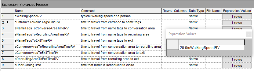
Figure 4.9: Defining the expressions for the revised STEM Mixer example
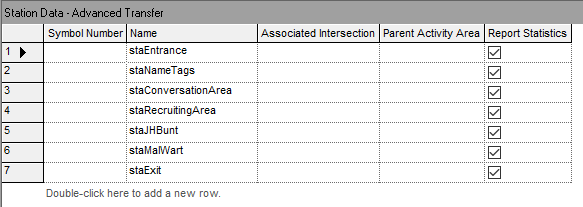
Figure 4.10: Defining the stations for the revised STEM Mixer example
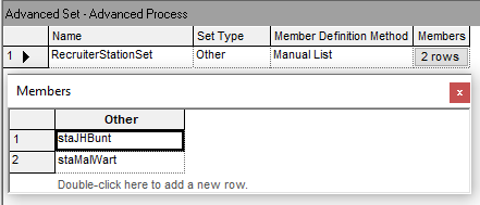
Figure 4.11: Defining the station set for the revised STEM Mixer example
To implement the flow chart modules, we can start with the creation of the students and the logical entity to shut off the creation of students at the appropriate time.
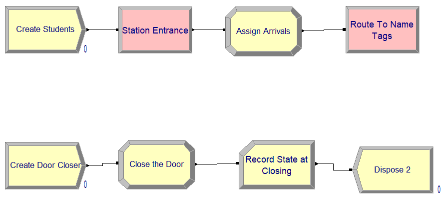
Figure 4.12: Creating the students and closing the doors

Figure 4.13: Data for CREATE modules
Figure 4.12 shows the flow chart modules for creating the students and the door closing entity, which map almost directly to the pseudo-code listings. Figure 4.13 shows the data view of the CREATE modules. Notice the use of the stream number in specifying the mean time between arrivals of the students and the use of the variable, vMaxArrivals, in the “Max Arrivals” field. The expression, eDoorClosingTime, is used to specify the time of the first creation for the door closing entity. Why use an expression for this time? As noted in Figure 4.9, the eDoorClosingTime expression is computed from the two variables, vWarningTime and vMixerTimeLength. Defining these as parameters to the model facilitates their use when performing experiments. This is also good model building practice. To the extent possible define parameters as variables or expressions. Do not embedded magic numbers (undocumented constants) within the text fields of the dialog boxes. After being created, the students go to the name tag are as illustrated in Figure 4.14. As noted in the pseudo-code, first we check if the mixer closed during the time that it took for the entity to get to the name tag area. If the mixer has not closed, the student decides whether or not to directly visit the recruiting area or the conversation area.
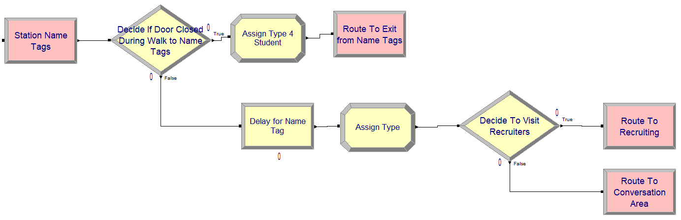
Figure 4.14: Name tag station and modules
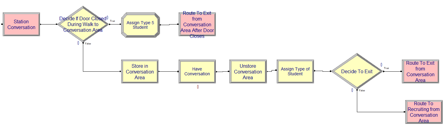
Figure 4.15: Conversation area station and modules
Those students that first go to the conversation area proceed to the logic illustrated in Figure 4.15. The other students go directly to the logic shown in Figure 4.16. Notice the use of the STORE and UNSTORE modules in Figure 4.16.
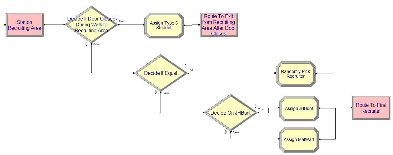
Figure 4.16: Recruiting area station and modules
Figure 4.16 shows the use of the DECIDE module to implement the logic associated with determining which recruiter is visited first. If there is a tie between the two recruiters, one of stations associated with the recruiters is randomly selected; otherwise, the station with the lower number of students is selected. Figure 4.17 shows the data view for all of the ROUTE modules in the model. Notice that the already discussed expressions are used in each of the ROUTE modules. In addition, the ROUTE module defined on line 11 implements the random selection of the station to visit by using the MEMBER() function. The Arena MEMBER(set name, set index) function will return the member of the set indicated by the index of the set member. In this case, the RecruiterStationSet is indexed into by the attribute myFirstRecruiter, which was assigned previously in one of the ASSIGN modules of Figure 4.16.
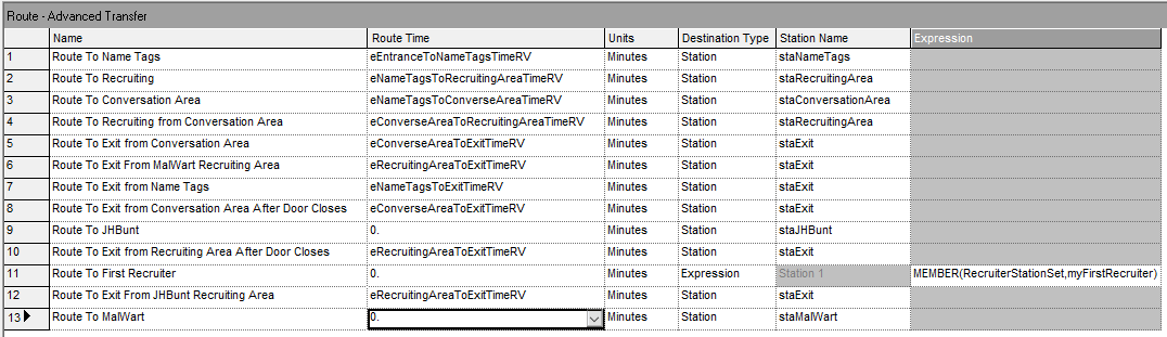
Figure 4.17: Data view for ROUTE modules
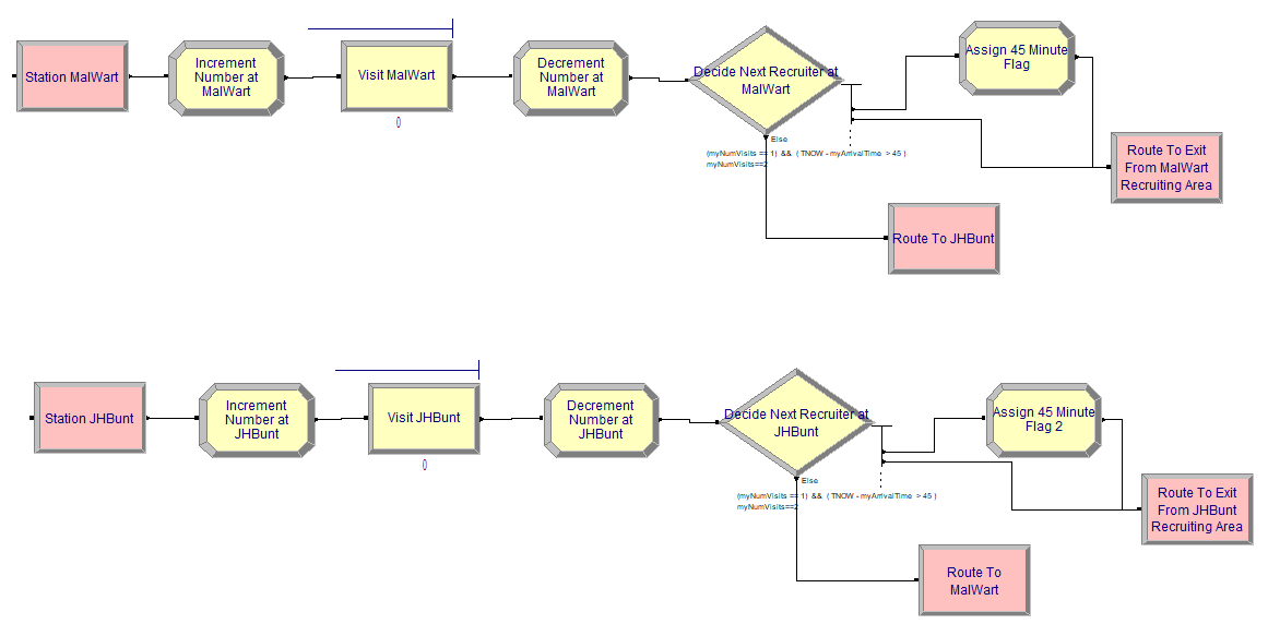
Figure 4.18: JHBunt and MalWart recruiting station modules
After selecting the recruiter to visit first, the students will go to either of the two stations shown in Figure 4.18. The logic associated with both stations is essentially the same. First the number of students at the recruiter is incremented, the student enters the recruiting process, and then the number of students at the recruiter is decremented. The entries for the two PROCESS modules show in Figure 4.18 are shown in Figure 4.19. Finally, an N-way by condition is used to implement the DECIDE logic for exiting or visiting the other recruiter. Notice that the distributions associated with the delay have been updated to utilize the required stream numbers.
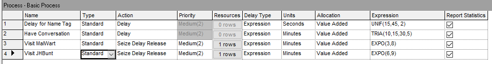
Figure 4.19: STEM Mixer PROCESS modules
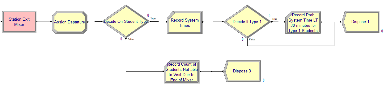
Figure 4.20: STEM Mixer exit station modules
After visiting the recruiter area, the students will depart. Figure 4.20 shows the layout of the modules to collect statistics on departing students. This logic has been simplified, as compared to, what was presented in Chapter 3 because of the use of tally sets. Figure x15 shows that a record can be defined that can collect statistics on the system time by type of student. This option is implemented by checking the “Record in Set” option for the RECORD module, designating the set containing the created tally variables, and defining the attribute that can be used to select the correct member from the set via the “Set Index” field.
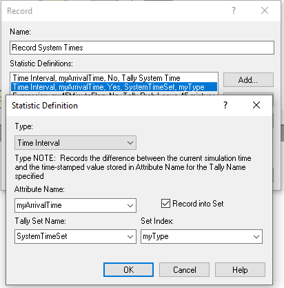
Figure 4.21: Recording the system times with a tally set
Running the model for 30 replications, we achieve the results shown in Figure 4.22 and Figure 4.23.
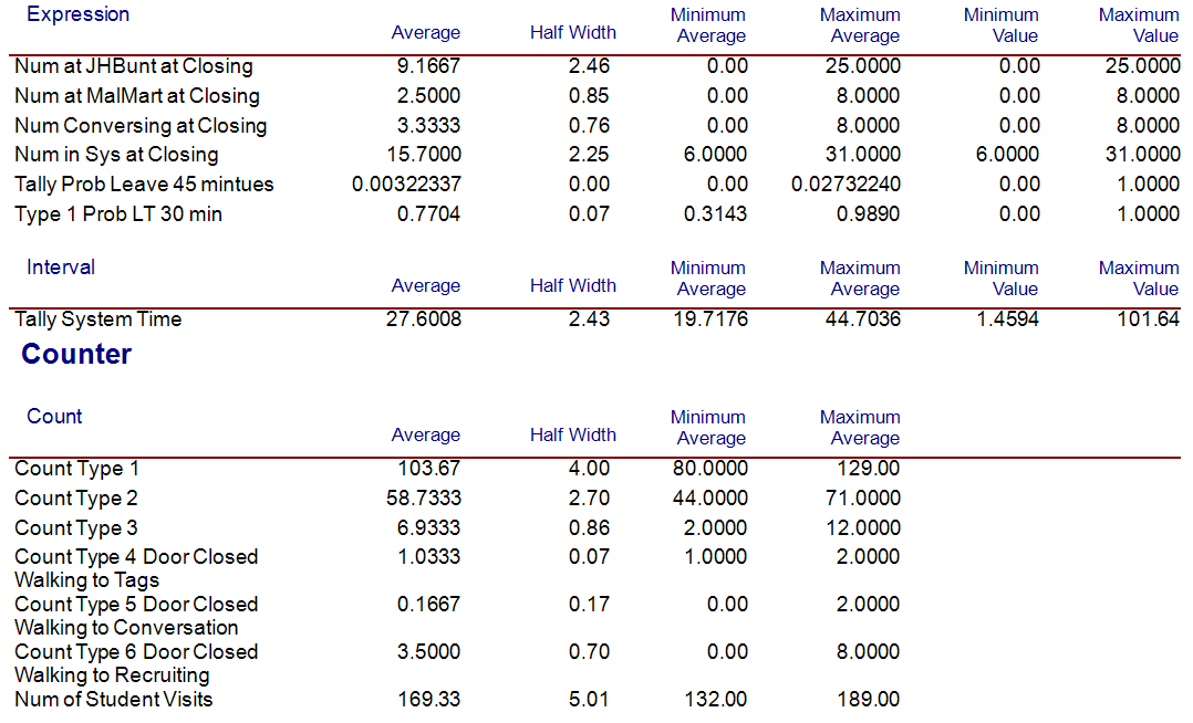
Figure 4.22: Results for closing statistics
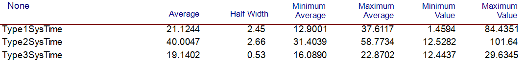
Figure 4.23: Results for system times by student type
Figure 4.23 shows the system times for the different types of students. A type 1 student goes directly to the recruiting area. A type 2 student first visits the conversation area before visiting the recruiting area. A type 3 student first visits the conversation area and then decides to directly depart the mixer. Figure 4.22 shows that there are on average about 15.7 students in the system when the closing starts. The probability that type 1 students spend less than 30 minutes attending the fair is about 77 percent on average.
In this section, we learned about the Arena elements: EXPRESSION, ROUTE, STATION, STORAGE, STORE, and UNSTORE. In particular, we saw how we can define expressions and use them throughout the model and represent the simple transfer of entities between locations with a time delay. In the next section, we build on some prior concepts, especially attributes, variables, and expressions to see how these concepts can be put to use within Arena. So far, our examples have shown situations where entities flow essentially forward through the model, perhaps taking different paths. In the next section, we illustrate how entities can be used to loop through Arena modules to implement coding logic. In addition, we see how arrays can facilitate model building and additional methods for organizing the modules within the flow chart area.