4.2 Example: Iterative Looping, Expressions, and Sub-models

In this example, we will work with attributes, variables, and expressions. The model will also introduce modules that facilitate iterative looping (while loops) that you would see in general purpose programming languages. In addition, we will see how Arena facilitates the use of arrays to hold variable values and expressions. The main purpose of this model is to illustrate how to use these programming constructs within an Arena model.

The model introduced in this section will use the following modules:

CREATE Two instances of this module will be used to have two different arrival processes into the model.
ASSIGN This module will be used to assign values to variables and attributes.
WHILE & ENDWHILE These modules will be used to loop the entities until a condition is true.
DECIDE This module will also be used to loop entities until a condition is true
PROCESS This module will be used to simulate simple time delays in the model.
DISPOSE This module will be use to dispose of the entities that were created.
VARIABLES This data module will be used to define variables and arrays for the model.
EXPRESSIONS This data module will be used to define named expression to be used within the model.
Sub-models are areas of the model window that contain modules that have been aggregated into one module.

This example is based partly on Arena’s SMARTS file 183. The final model will look something like that shown in Figure 4.24.

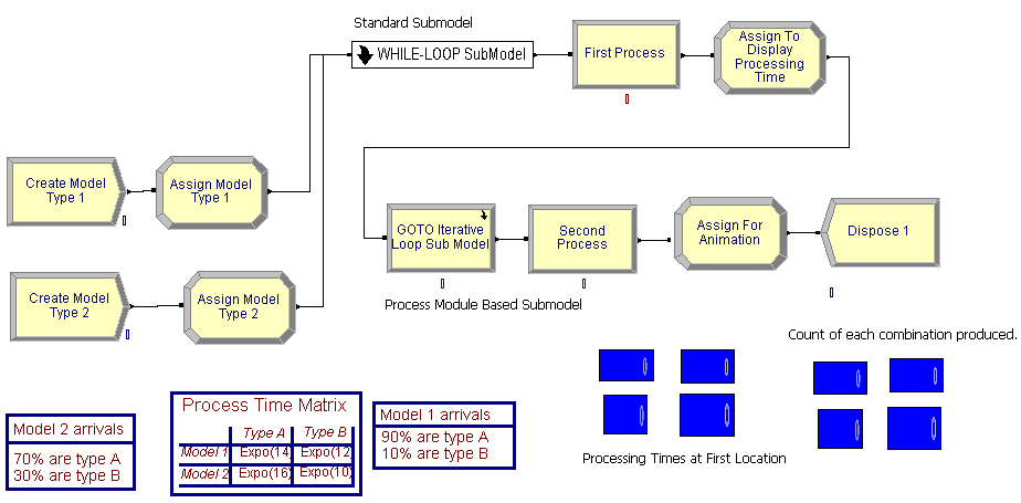
Figure 4.24: Completed model for iterative looping example

This system produces products. The products have different model configurations (model 1 and 2) that are being produced within a small manufacturing system. Model 1 arrives according to a Poisson process with a mean rate of 1 model every 12 minutes. The second model type also arrives according to a Poisson arrival process but with a mean arrival rate of 1 arrival every 22 minutes. Furthermore, within a model configuration, there are two types of products produced, type A and type B.

Table 4.1 shows the data for this example. In the table, 90% of model configuration 1 is of type A. In addition, the base process time for type A’s for model configuration 1 is exponentially distributed with a mean of 14 minutes. Clearly, the base process time for the products depends on the model configuration and the type of product A or B. The actual processing time is the sum of 10 random draws from the base distribution. Processing occurs at two identical sequential locations. After the processing is complete, the product leaves the system.

Table 4.1: Data for the iterative looping example
Model	Mean Rate	Type A(%, process time)	Type B(%, process time)
1	1 every 12 minutes	90%, expo(14) minutes	10%, expo(12) minutes
2	1 every 22 minutes	70%, expo(16) minutes	30%, expo(10) minutes

When building this model, we will display the final processing time for each product at each of the two locations and display a count of the number of each configuration and type that was produced.

4.2.0.1 Building the Model

Following the basic modeling recipe, consider the question: What are the entities? By definition, entities are things that flow through the system. They are transient. They are created and disposed. For this situations, the products are produced by the system. The products flow through the system. These are definite candidates for entities. In this problem, there are actually four types of entities: Two main types Model 1 and Model 2, which are further classified into product type A or product type B. Now, consider how to represent the entity types. This can be done in two ways 1) by using the ENTITY module to define an entity type or 2) by using user defined attributes. Either method can be used in this situation, but by using user defined attributes, we can more easily facilitate some of the answers to some of the other modeling recipe questions.

Now, it is time to address the question: What are the attributes of the entities? This question is partly answered already by the decision to use user defined attributes to distinguish between the types of entities. Let’s define two attributes, myModel and myType to represent the classification by model and by product type for the entities. For example, if myModel = 1 then the entity is of type model configuration 1. To continue addressing the required attributes, you need to consider the answers to:

What data do the entities need as they move through the model? Can they carry the data with them as they move or can the information be shared across entities?
What data belongs to the system as a whole?

The answer to the first question is that the parts need their processing times. The answer to the second question can have multiple answers, but for this model, the distributions associated with the processing times need to be known and this information doesn’t change within the model. This should be a hint that it can be stored globally. In addition, the processing time needs to be determined based on different distributions at each of the two locations.

While you might first think of using variables to represent the processing time at each location, you will soon realize that there is a problem with this approach. Assume that a variable holds the processing time for the entity that is currently processing at location 1. While that entity is processing, another entity can come along and over write the variable. This is clearly a problem. The better approach is to realize that the entities can carry their processing times with them after the processing times have been computed. This should push you toward the use of an attribute to hold the processing time. Let’s decide to have an attribute called myProcessingTime that can be used to hold the computed processing time for the entity before it begins processing. If data is not to be carried by the entities, but it still needs to be accessed, then this is a hint that it belongs to the system as a whole. In this case, the processing time distributions need to be accessed by any potential entity.

How can the entities be created? The problem description gives information about two Poisson arrival processes. While there are other ways to proceed, the most straightforward approach is to use a CREATE module for each arrival process. If this is done, one CREATE module will create the entities having model configuration 1 and the other CREATE module will create the entities having model configuration 2. How do you assign data to the entities? An ASSIGN module can be used for this task, but more importantly, the model configuration, the product type, and the processing time all will need to be assigned. In particular, the product type can be randomly assigned according to a given distribution based on the model configuration. In addition, the processing time is the sum of 10 draws from the processing time distribution. Thus, a way to compute the final processing time for the entity before it starts processing must be determined.

The following pseudo-code for the example is as follows. First, we define the attributes, variables and expressions. For variables, we see something new. We have defined a 2-dimensional variable called vMTCount that will be used to count the number of parts of each model and type combination that are produced. This 2-dimensional variable can be used just like in other programming languages. Similarly, we define a 2-dimensional expression. Just like was illustrated in the last example, an expression can hold any valid Arena expression; however, in this case, we have defined an arrayed expression from which we can look up the appropriate distribution associated with a particular model and product type combination. This is an extremely useful method to store information.

// Model Definition Pseudo-Code
ATTRIBUTES:
myType // represents the type of product, 1 = type A, 2 = type B
myModel // represents the type of model, 1 = Model Type 1, 2 = Model Type 2
myProcessingTime // holds the total processing time based on the model/product type
VARIABLES:
vCounter = 0 // used to count the number of iterations in a loop
vNumIterations = 10 // represents the total number of iterations in a loop
vMTCount: 2-D Array, rows = 2 (model type), columns = 2 (product type)
  vMTCount(1,1) = 0, vMCount(1,2) = 0
  vMTCount(2,1) = 0, vMCount(2,2) = 0
vPTLocation1: 2-D Array, rows = 2 (model type), columns = 2 (product type)
  vPTLocation1(1,1) = 0, vPTLocation1(1,2) = 0
  vPTLocation1(2,1) = 0, vPTLocation1(2,2) = 0
vPTLocation2: 2-D Array, rows = 2 (model type), columns = 2 (product type)
  vPTLocation2(1,1) = 0, vPTLocation2(1,2) = 0
  vPTLocation2(2,1) = 0, vPTLocation2(2,2) = 0

EXPRESSIONS:
// represents the processing time distribution for model and product type combinations
ePTIme: 2-D Array, rows = 2 (model type), columns = 2 (product type)
  ePTime(1,1) = EXPO(14), ePTime(1,2) = EXPO(12)
  ePTime(2,1) = EXPO(16), ePTime(2,2) = EXPO(10)

After defining the constructs to use, we can then outline the processes within pseudo-code. We start with the creation of the two types of model configurations and the assignment of the product types. After creation the entities will have their model and type assigned. Then, they will proceed for processing. Prior to processing at the first station, the processing time is determined. In the pseudo-code, a WHILE-ENDWHILE construct is used to sum up the processing time. After the processing time has been determined, the entity delays for the processing time. After the processing is done at the first station, the processing time for the second station is computed. Here the processing time is determined in an iterative fashion by using a go to construct coupled with an if statement. After the processing time has been determined, the entity again delays for the processing before being disposed.

CREATE 10 entities with TBA EXPO(12) 
ASSIGN model 1 attributes 
  myModel = 1
  myType = DISC(.9,1,1,2)
END ASSIGN
GOTO label A 

CREATE 10 entities with TBA EXPO(22)
ASSIGN model 2 attributes 
   myModel = 2 
   myType = DISC(.7,1,1,2)
END ASSIGN
GOTO label A

Label A: determine the processing time for first station 
BEGIN ASSIGN //initialize the loop
  vCounter = 1 
  vNumIterations = 10
  myProcessingTime = 0
END ASSIGN
WHILE (vCounter <= vNumIterations)
  BEGIN ASSIGN
    // sum up the processing time by model and product type
    myProcessingTime = myProcessingTime + ePTime(myModel, myType)
    vCounter=vCounter + 1 //increment the counter
  END ASSIGN
ENDWHILE
DELAY for myProcessingTime
BEGIN ASSIGN //initialize the loop for second station
  vCounter = 0 
  vNumIterations = 10
  myProcessingTime = 0
END ASSIGN
Label B:
BEGIN ASSIGN
  // sum up the processing time by model and product type
  myProcessingTime = myProcessingTime + ePTime(myModel, myType)
  vCounter=vCounter + 1 //increment the counter
END ASSIGN
DECIDE IF (vCounter <= vNumIterations)
  GOTO Label B
END DECIDE
DELAY for myProcessingTime
DISPOSE

The model will follow the outline presented within the pseudo-code. To support the modeling within the environment, you must first define a number of variables and other data.

4.2.0.2 VARIABLE Module

Begin by defining the variables to be used in the model. Open the environment and define following variables using the VARIABLE module as shown in Figure 4.25.

vCounter used to count the number of times the entity goes through the WHILE-ENDWHILE loop, a scalar variable. This WHILE-ENDWHILE loop will be used to compute the processing time at each location.
vNumIterations used to indicate the total number of times to go through the WHILE-ENDWHILE loop, a scalar variable. This should be initialized to the value 10.
vMTCount used to assist with counting and displaying the number of entities of each model/type combination, a 2-dimensional variable (2 rows, 2 columns)
vPTLocation1 used to assist with displaying the processing time of each model/type combination, a 2-dimensional variable (2 rows, 2 columns)
vPTLocation2 used to assist with displaying the processing time of each model/type combination, a 2-dimensional variable (2 rows, 2 columns)

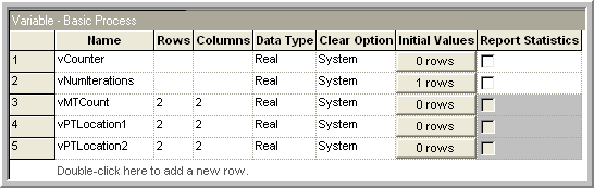
Figure 4.25: Variable definitions for iterative looping example

The example specifies that there is a different distribution for each model/product type combination. Thus, we need to be able to store these distributions. A distribution is considered a mathematical expression. A list of distributions is found in Table E.3 in Appendix E. In the table, the function name is given along with the parameters required by the function. The Stream parameter indicates an optional parameter which helps in controlling the randomness of the distribution. In addition to using distributions in expressions, you can use logical constructs and mathematical operators to build expressions. Table E.1 of Appendix E provides a list of mathematical functions available. To represent the model/product type distributions, the EXPRESSION data module can be used.

4.2.0.3 EXPRESSION Module

While you can build expressions using the previously mentioned functions and operators, a mechanism is needed to ’hold the expressions in memory, and in particular, for this problem, the appropriate distribution must be looked up based on the model type and the product type. The EXPRESSION module found on the Advanced Process template allows just this functionality. Expressions as defined in an EXPRESSION module are names or labels assigned to expressions. An expression defined in an EXPRESSION module is substituted wherever the named expression appears in the model. The EXPRESSION module also allows for the modeler to define an array of expressions.

Go to the Advanced Process panel and define the expressions used in the model by clicking on the EXPRESSION module in the project bar, defining the name of the expression, ePTime, to have two rows and two columns, where the row designates the model type and the column designates the product type. Use the spreadsheet view to enter the exponential distribution with the appropriate mean values as indicated in Figure 4.26.

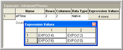
Figure 4.26: Expression definitions for iterative looping example

This creates an arrayed expression. This is similar to an arrayed variable, except that the value stored in the array element can be any valid expression. Now that you have the basic data predefined for the model you can continue with the model building by starting with the CREATE modules. Since the model is large, you will begin by laying down the first part of the model. You should place the two CREATE modules and the two ASSIGN modules into the model window as shown in Figure 4.24. Fill in the create modules as indicated in Figure 4.27. For this example, there will only be 10 products of each model configuration created.

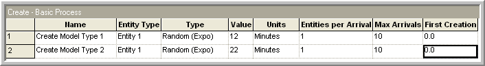
Figure 4.27: Creating the products for iterative looping example

The ASSIGN modules can be used to define the attributes and to assign their values. In the ASSIGN modules, the values of the myModel and myType attributes are assigned. There are two different models 1 and 2. Also, each model is assigned a type, dependent upon a specific probability distribution for that model. The DISC() function can be used to represent the model type. Open up the first ASSIGN module for model type 1 and make it look like the ASSIGN module show in Figure 4.28.

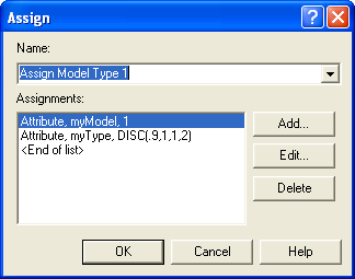
Figure 4.28: ASSIGN module dialog box for model type 1

For variety, you can use the spreadsheet view to fill out the second ASSIGN module. Click on the ASSIGN module in the model window. The corresponding ASSIGN module will be selected in the data sheet view. Click on the assignment rows to get the assignments window and fill it in as indicated in Figure 4.29.

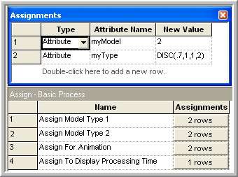
Figure 4.29: Second ASSIGN module in data sheet view

4.2.0.4 Hierarchical Sub-models

In this section, the middle portion of the model as indicated in Figure 4.30, which includes a sub-model will be built. A sub-model in is a named collection of modules that is used to organize the main model. Go to the Object menu and choose Sub-model \(>\) Add Sub-model. Place the cross-haired cursor that appears in the model window at the desired location and connect your ASSIGN modules to it as indicated in the figure. By right-clicking on the sub-model and selecting the properties menu item, you can give the sub-model a name. This sub-model will demonstrate the use of a WHILE-ENDWHILE loop. The WHILE-ENDWHILE construct will be used as an iterative looping technique to compute the total processing time according to the number of iterations (10) for the given model/type combination.

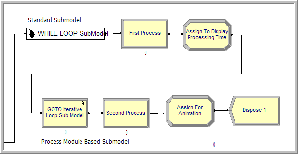
Figure 4.30: First location processing

4.2.0.5 WHILE-ENDWHILE Blocks

Open up the sub-model by double clicking on it and add the modules (ASSIGN, WHILE, ASSIGN, and ENDWHILE) to the sub-model as indicated in Figure 4.31. You will find the WHILE and ENDWHILE blocks on the BLOCKS panel. If you haven’t already done so you should attach the BLOCKS panel by going to the Basic Process panel and right clicking, choose Attach, and then select the file called Blocks.tpo. A new panel of blocks will appear for use.

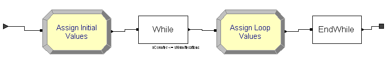
Figure 4.31: First location processing sub-model

Now we implement the pseudo-code logic within the sub-model. We will initialize the counter in the first Assign block:

The counter can be an attribute or a variable
If the counter is an attribute, then every entity has this attribute and the value will persist with the entity as it moves through the model. It may be preferable to have the counter as an attribute for the reason given in item (3) below.
If the counter is a (global) variable, then it is accessible from anywhere in the model. If the WHILE-ENDWHILE loop contains a block that can cause the entity to stop moving (e.g. DELAY, HOLD, etc. then it may be possible for another entity to change the value of the counter when the entity in the loop is in the delayed state. This may cause unintended side effects, e.g. resetting the counter would cause an infinite loop. Since there are no time delays within this WHILE-ENDWHILE loop example, there is no danger of this. Remember, there can only be one entity moving (being processed by the simulation engine) at anytime while the simulation is running.

Open up the first ASSIGN module and make it look like that shown in Figure 4.32. Notice how the variables are initialized prior to the WHILE. In addition, the myProcessingTime attribute has been defined and initialized to zero.

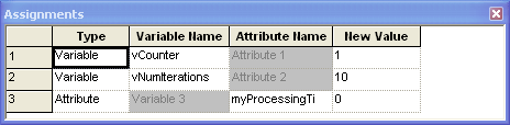
Figure 4.32: Initializing the looping counter

Now the counter must be checked in the condition expression of the WHILE block. The WHILE and ENDWHILE blocks can be found on the Blocks Panel. Open up the WHILE block and make it look like that shown in Figure 4.33. When the variable vCounter is greater than vNumIterations, the WHILE condition will evaluate to false and the entity will exit the WHILE-ENDWHILE loop.

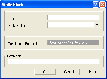
Figure 4.33: WHILE block within first sub-model

Make sure to update the value of the counter variable or the evaluation expression within the body of the WHILE and ENDWHILE loop; otherwise you may end up with an infinite loop. Open up the second ASSIGN module and make the assignments as shown in Figure 4.34. In the first assignment, the attributes myModel and myType are used to index into the ePTime array of expressions. Each time the entity hits this assignment statement, the value of the myProcessingTime attribute is updated based on the previous value, resulting in a summation. The variable vCounter is incremented each time to ensure that the WHILE loop will eventually end.

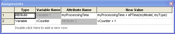
Figure 4.34: Second ASSIGN module with first sub-model

There is nothing to fill in for the ENDWHILE block. Just make sure that it is connected to the last ASSIGN module and to the exit point associated with the sub-model. Right clicking within the sub-model will give you a context menu for closing the sub-model. After the entity has exited the sub-model, the appropriate amount of processing time has been computed within the attribute, myProcessingTime. You now need to implement the delay associated with processing the entity for the computed processing time.

4.2.0.6 PROCESS Module Delay Option

Within only the active entity is moving through the modules at any time. The active entity is the entity that the simulation executive has determined is associated with the current event. At the current event time, the active entity executes the modules along its flow path until it is delayed or cannot proceed due to a condition in the model. When the active entity is time delayed, an event is placed on the event calendar that represents the time that the delay will end. In other words, a future event is scheduled to occur at the end of the delay. The active entity is placed in the future events list and yields control to the next entity that is scheduled to move within the model. The simulation executive then picks the next event and the associated entity and tells that entity to continue executing modules. Thus, only one entity is executing model statements at the current time and that module execution only occurs at event times. moves from event time to event time, executing the associated modules. This concept is illustrated in Figure 4.35 where a simple delay is scheduled to occur in the future. It is important to remember that while the entity associated with the delay is waiting for its delay to end, other events may occur causing other entities to move.

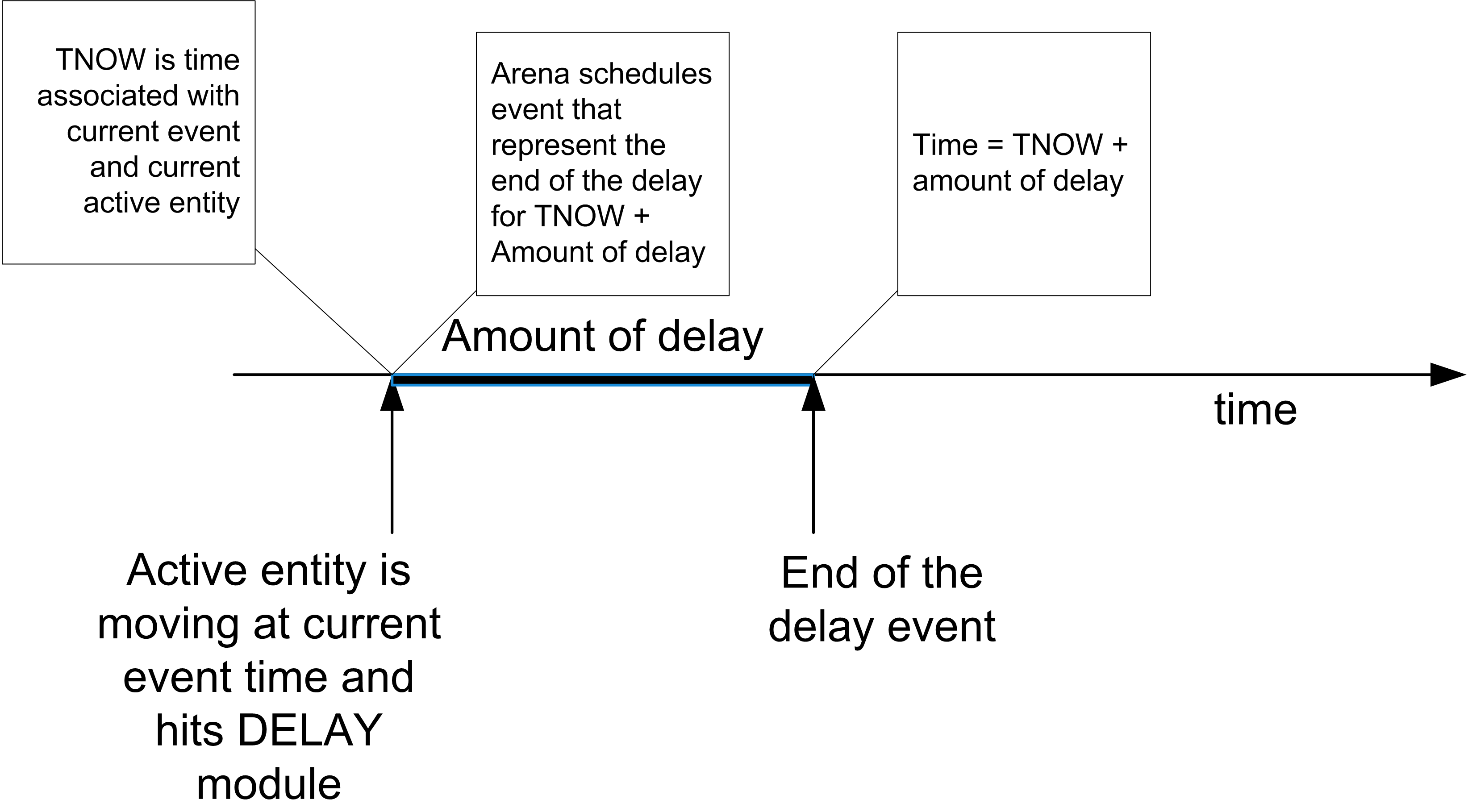
Figure 4.35: Scheduling a selay

There are two basic ways to cause a delay for an entity, the PROCESS module and the DELAY module. We have already used the delay option of the PROCESS module. The DELAY module is found on the Advanced Process template panel. This example illustrates the use of the DELAY module. The next step in building the model is to place the DELAY module after the sub-model as shown in Figure 4.30. In this case, you want to delay by the amount of time computed for the processing time. This value is stored in the myProcessingTime attribute. Within the expression text field fill in myProcessingTime as shown in Figure 4.36. Be careful to appropriately set the time units (minutes) associated with the delay. A common mistake is to not set the units and have too long or too short a delay. The too long a delay is often caught during debugging because the entities take such a long time to leave the module.

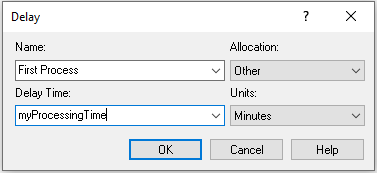
Figure 4.36: The DELAY module

Now you will add an ASSIGN module to facilitate the displaying of the values of variables in the model window during the simulation. This will also illustrate how arrays can be used within a model. Using the data sheet view, make the ASSIGN module look like that show in Figure 4.37.

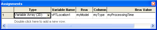
Figure 4.37: ASSIGN module with arrays

The values of attributes cannot be displayed using the variable animation constructs. So, in this ASSIGN module, an array variable is used to temporarily assign the value of the attribute to the proper location of the array variable so that it can be displayed. Go to the toolbar area in and right click. Make sure that the Animate toolbar is available. From the Animate toolbar, choose the button that has a 0.0 indicated on it. You will get a dialog for entering the variable to display. Fill out the dialog box so that it looks like Figure 4.38. After filling out the dialog and choosing OK, you will need to place the cross-hair somewhere near the ASSIGN module in the model window. In fact, the element can be placed anywhere in the model window. Repeat this process for the other elements of the vPTLocation1 array.

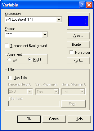
Figure 4.38: Animate variable dialog box

Now, the model can be completed. Lay down the modules indicated in Figure 4.24 to complete the model. In Figure 4.24, the second sub-model uses a PROCESS based sub-model. It looks like a PROCESS module and is labeled "GOTO Iterative Loop Sub Model", see Figure 4.39. To create this sub-model, lay down a PROCESS module and change its type to sub-model. In what follows, you will examine a different method for looping within the second sub-model. Other than that, the rest of the model is similar to what has already been completed. The second sub-model has the modules given in Figure 4.40. Place and connect the ASSIGN, DECIDE, and ASSIGN modules as indicated in Figure 4.41 and Figure 4.42. In this logic, the entity initializes a counter for counting the number of times through the loop and updates the counter. An If/Then DECIDE module is used to redirect the entity back through the loop the appropriate number of times. This is GOTO programming!

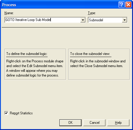
Figure 4.39: PROCESS based sub-model

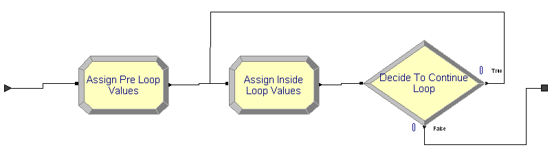
Figure 4.40: Second sub-model modules

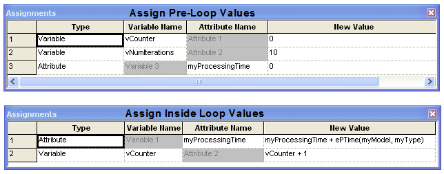
Figure 4.41: ASSIGN modules in second sub-model

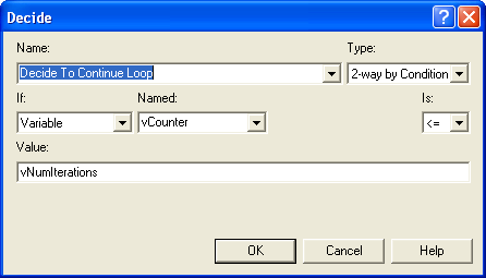
Figure 4.42: ASSIGN modules in second sub-model

Again, be sure to use logic that will change the tested condition (in this case vCounter) so that you do not get an infinite loop. I prefer the use of the WHILE-ENDWHILE blocks instead of this “go to” oriented implementation, but it is ultimately a matter of taste.

In general, you should be careful when implementing logic in which the entity simply loops around to check a condition. As mentioned, you must ensure that the condition can change to prevent an infinite loop. A common error is to have the entity check a condition that can be changed from somewhere else in the model, e.g. a queue becomes full. Suppose you have the entity looping around to check if the queue is not full so that when the queue becomes full the entity can perform other logic. This seems harmless enough; however, if the looping entity does not change the status of the queue then it will be in an infinite loop! Why? While you might have many entities in the model at any given simulated time, only one entity can be active at any time. You might think that one of the other entities in the model may enter the queue and thus change its status. If the looping entity does not enter a module that causes it to “hand off the ball” to another entity then no other entity will be able to move to change the queue condition. If this occurs, you will have an infinite loop.

If the looping entity does not explicitly change the checked condition, then you must ensure that the looping entity passes control to another entity. How can this be achieved? The looping entity must enter a blocking module that allows another entity to get to the beginning of the future events list and become the active entity. A blocking module is a module that causes the forward movement ofan entity to stop in some manner. There are a variety of modules which will cause this, e.g. HOLD, SEIZE, DELAY, etc. Another thing to remember, even if the looping entity enters a blocking module, your other simulation logic must ensure that it is at least possible to have the condition change. If you have a situation where an entity needs to react to a particular condition changing in the model, then you should consider investigating the HOLD and SIGNAL modules, which were designed specifically for these types of situations.

The second DELAY module is exactly the same as the first DELAY module. In fact, you can just copy the first DELAY module and paste the copy into the model at the appropriate location. If you do copy and paste a module in this fashion, you should make sure to change the name of the module because module names must be unique. The last ASSIGN module is just like the previously explained example. Complete the ASSIGN module as shown in Figure 4.43. Complete the animation of the model in a similar fashion as you did to show the processing time at the first location, except in this case show the counts captured by the variable vMTCount.

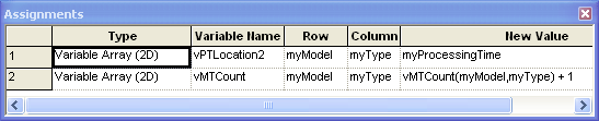
Figure 4.43: Last ASSIGN module for animation purposes

To run the model, execute the model using the “VCR” run button. It is useful to use the step command to track the entities as they progress through model. You will be able to see that the values of the variables change as the entities go through the modules. The completed model can be found in the files associated with this chapter as file AttributesVariablesExpressionsLooping.doe.

To recap, in this example you learned about attributes and how they are attached to entities. In addition, you saw how to share global information through the use of arrays of variables and arrays of expressions. The concept of scheduling events via the use of the DELAY module was also introduced. Finally, you also refreshed your memory on basic programming constructs such as decision logic and iterative processing.