3.2 Types of Statistical Quantities in Simulation
A simulation experiment occurs when the modeler sets the input parameters to the model and executes the simulation. This causes events to occur and the simulation model to evolve over time. This execution generates a sample path of the behavior of the system. During the execution of the simulation, the generated sample path is observed and various statistical quantities computed. When the simulation reaches its termination point, the statistical quantities are summarized in the form of output reports.
A simulation experiment may be for a single replication of the model or may have multiple replications. As previously noted, a replication is the generation of one sample path which represents the evolution of the system from its initial conditions to its ending conditions. If you have multiple replications within an experiment, each replication represents a different sample path, starting from the same initial conditions and being driven by the same input parameter settings. Because the randomness within the simulation can be controlled, the underlying random numbers used within each replication of the simulation can be made to be independent. Thus, as the name implies, each replication is an independently generated “repeat” of the simulation. Figure 1.2 illustrates the concept of replications being repeated (independent) sample paths.
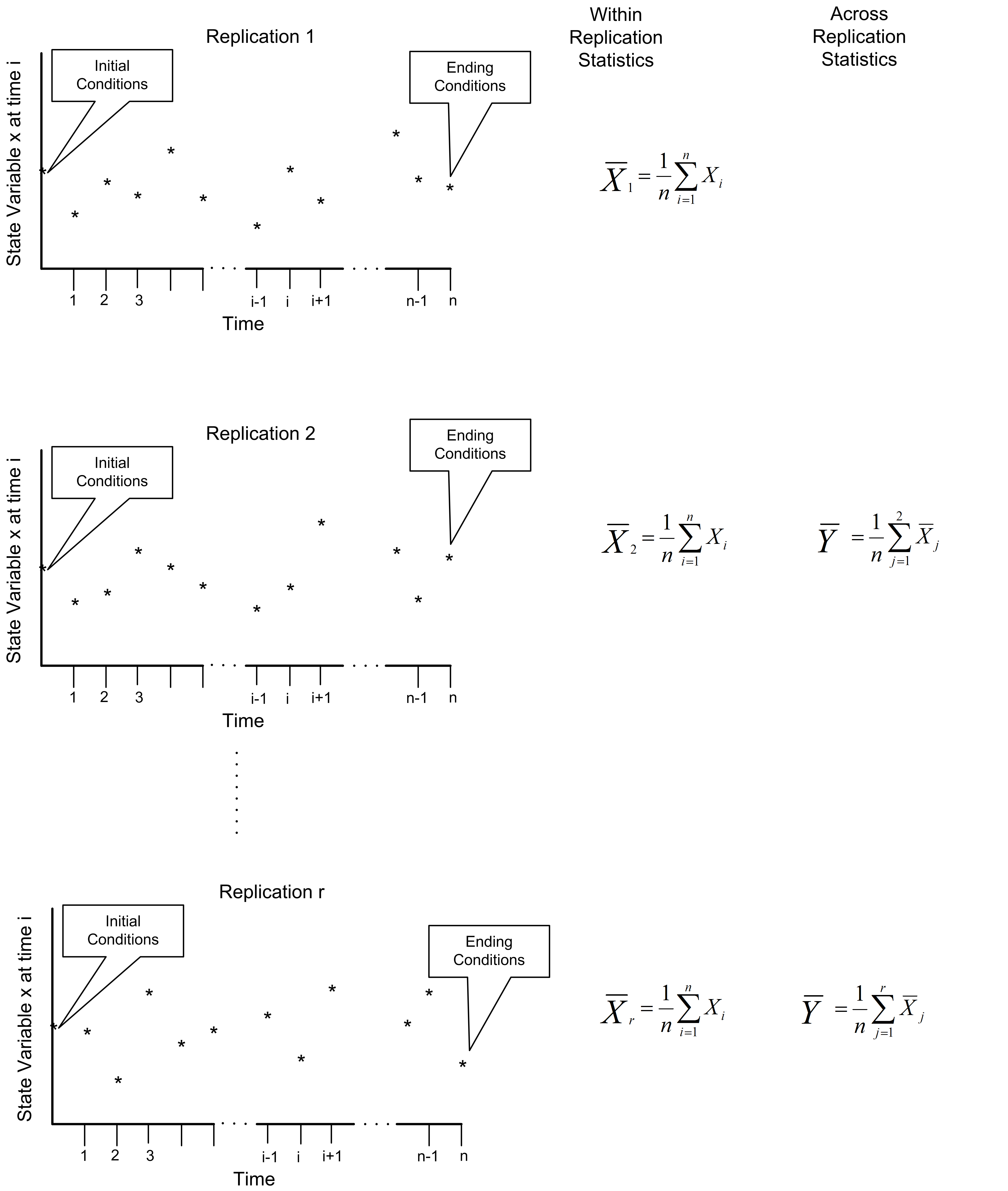
Figure 3.2: The concept of replicated sample paths
3.2.1 Within Replication Observations
Within a single sample path (replication), the statistical behavior of the model can be observed. The statistical quantities collected during a replication are called within replication statistics.
Within replication statistics are collected based on the observation of the sample path and include observations on entities, state changes, etc. that occur during a single sample path execution. The observations used to form within replication statistics are not likely to be independent and identically distributed.
For within replication statistical collection there are two primary types of observations: tally and time-persistent. Tally observations represent a sequence of equally weighted data values that do not persist over time. This type of observation is associated with the duration or interval of time that an object is in a particular state or how often the object is in a particular state. As such it is observed by marking (tallying) the time that the object enters the state and the time that the object exits the state. Once the state change takes place, the observation is over (it is gone, it does not persist, etc.). If we did not observe the state change when it occurred, then we would have missed the observation. The time spent in queue, the count of the number of customers served, whether or not a particular customer waited longer than 10 minutes are all examples of tally observations. The vast majority of tally based data concerns the entities that flow through the system.
Time-persistent observations represent a sequence of values that persist over some specified amount of time with that value being weighted by the amount of time over which the value persists. These observations are directly associated with the values of the state variables within the model. The value of a time-persistent observation persists in time. For example, the number of customers in the system is a common state variable. If we want to collect the average number of customers in the system over time, then this will be a time-persistent statistic. While the value of the number of customers in the system changes at discrete points in time, it holds (or persists with) that value over a duration of time. This is why it is called a time-persistent variable.
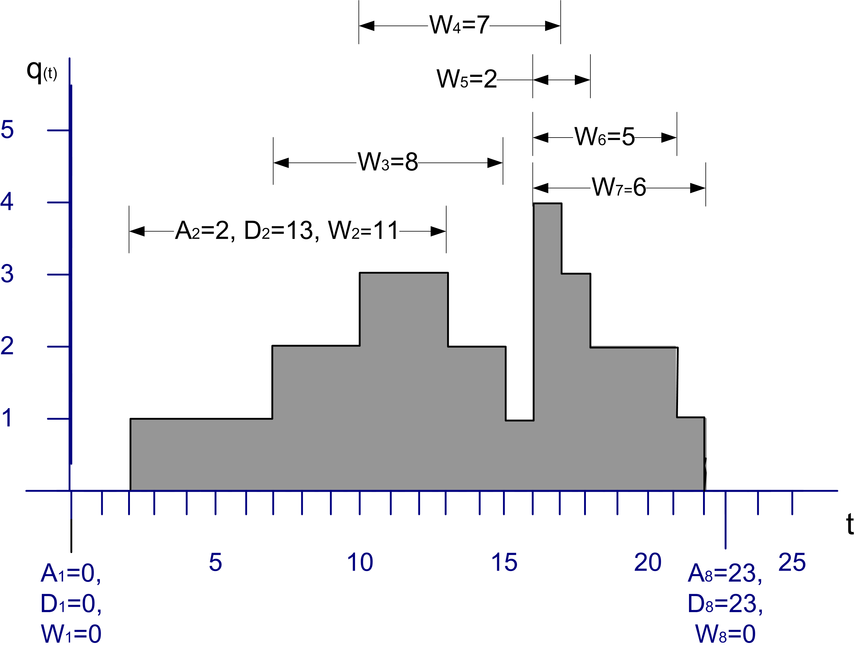
Figure 3.3: Sample path for tally and time-persistent data
Figure 3.3 illustrates a single sample path for the number of customers in a queue over a period of time. From this sample path, events and subsequent statistical quantities can be observed. Let’s define some variables based on the data within Figure 3.3.
Let \(A_i \; i = 1 \ldots n\) represent the time that the \(i^{th}\) customer enters the queue
Let \(D_i \; i = 1 \ldots n\) represent the time that the \(i^{th}\) customer exits the queue
Let \(W_i = D_i - A_i \; i = 1 \ldots n\) represent the time that the \(i^{th}\) customer spends in the queue
Thus, \(W_i \; i = 1 \ldots n\) represents the sequence of wait times for the queue, each of which can be individually observed and tallied. This is tally type data because the customer enters a state (the queued state) at time \(A_i\) and exits the state at time \(D_i\). When the customer exits the queue at time \(D_i\), the waiting time in queue, \(W_i = D_i - A_i\) can be observed or tallied. \(W_i\) is only observable at the instant \(D_i\). This makes \(W_i\) tally based data and, once observed, its value never changes again with respect to time. Tally data is most often associated with an entity that is moving through states that are implied by the simulation model. An observation becomes available each time the entity enters and subsequently exits the state.
With tally data it is natural to compute the sample average as a measure of the central tendency of the data. Assume that you can observe \(n\) customers entering and exiting the queue, then the average waiting time across the \(n\) customers is given by:
\[\bar{W}(n) = \frac{1}{n}\sum_{i=1}^{n}W_{i}\]
Many other statistical quantities, such as the minimum, maximum, and sample variance, etc. can also be computed from these observations. Unfortunately, within replication data is often (if not always) correlated with respect to time. In other words, within replication observations like, \(W_i \, i = 1 \ldots n\), are not statistically independent. In fact, they are likely to also not be identically distributed. Both of these issues will be discussed when the analysis of infinite horizon or steady state simulation models is presented in Chapter 5.
The other type of statistical quantity encountered within a replication is based on time-persistent observations. Let \(q(t), t_0 < t \leq t_n\) be the number of customers in the queue at time \(t\). Note that \(q(t) \in \lbrace 0,1,2,\ldots\rbrace\). As illustrated in Figure 3.3, \(q(t)\) is a function of time (a step function in this particular case). That is, for a given (realized) sample path, \(q(t)\) is a function that returns the number of customers in the queue at time \(t\).
The mean value theorem of calculus for integrals states that given a function, \(f(\cdot)\), continuous on an interval \([a, b]\), there exists a constant, \(c\), such that
\[\int_a^b f(x)\mathrm{d}x = f(c)(b-a)\]
The value, \(f(c)\), is called the mean value of the function. A similar function can be defined for \(q(t)\). In simulation, this function is called the time-average or time-weighted average:
\[\bar{L}_q(n) = \frac{1}{t_n - t_0} \int_{t_0}^{t_n} q(t)\mathrm{d}t\]
This function represents the average with respect to time of the given state variable. This type of statistical variable is called time-persistent because \(q(t)\) is a function of time (i.e. it persists over time).
In the particular case where \(q(t)\) represents the number of customers in the queue, \(q(t)\) will take on constant values during intervals of time corresponding to when the queue has a certain number of customers. Let \(q(t)\) = \(q_k\) for \(t_{k-1} \leq t \leq t_k\) and define \(v_k = t_k - t_{k-1}\) then the time-average number in queue can be rewritten as follows:
\[\begin{aligned} \bar{L}_q(n) &= \frac{1}{t_n - t_0} \int_{t_0}^{t_n} q(t)\mathrm{d}t\\ & = \frac{1}{t_n - t_0} \sum_{k=1}^{n} q_k (t_k - t_{k-1})\\ & = \frac{\sum_{k=1}^{n} q_k v_k}{t_n - t_0} \\ & = \frac{\sum_{k=1}^{n} q_k v_k}{\sum_{k=1}^{n} v_k}\end{aligned}\]
Note that \(q_k (t_k - t_{k-1})\) is the area under \(q(t)\) over the interval \(t_{k-1} \leq t \leq t_k\) and
\[t_n - t_0 = \sum_{k=1}^{n} v_k = (t_1 - t_0) + (t_2 - t_1) + \cdots (t_{n-1} - t_{n-2}) + (t_n - t_{n-1})\]
is the total time over which the variable is observed. Thus, the time average is simply the area under the curve divided by the amount of time over which the curve is observed. From this equation, it should be noted that each value of \(q_k\) is weighted by the length of time that the variable has the value. This is why the time average is often called the time-weighted average. If \(v_k = 1\), then the time average is the same as the sample average.
With time-persistent data, you often want to estimate the percentage of time that the variable takes on a particular value. Let \(T_i\) denote the total time during \(t_0 < t \leq t_n\) that the queue had \(q(t) = i\) customers. To compute \(T_i\), you sum all the rectangles corresponding to \(q(t) = i\), in the sample path. Because \(q(t) \in \lbrace 0,1,2,\ldots\rbrace\) there are an infinite number of possible value for \(q(t)\) in this example; however, within a finite sample path you can only observe a finite number of the possible values. The ratio of \(T_i\) to \(T = t_n - t_0\) can be used to estimate the percentage of time the queue had \(i\) customers. That is, define \(\hat{p}_i = T_i/T\) as an estimate of the proportion of time that the queue had \(i\) customers during the interval of observation. Let’s take a look at an example.
Reviewing Figure 3.3 indicates the changes in queue length over a simulated period of 25 time units. Since the queue length is a time-persistent variable, the time average queue length can be computed as:
\[\begin{aligned} \bar{L}_q & = \frac{0(2-0) + 1(7-2) + 2(10-7) + 3(13-10) + 2(15-13) + 1(16-15)}{25}\\ & + \frac{4(17-16) + 3(18-17) + 2(21-18) + 1(22-21) + 0(25-22)}{25} \\ & = \frac{39}{25} = 1.56\end{aligned}\]
To estimate the percentage of time that the queue had \(\lbrace 0, 1, 2, 3, 4\rbrace\) customers, the values of \(v_k = t_k - t_{k-1}\) need to be summed for whenever \(q(t) \in \lbrace 0, 1, 2, 3, 4 \rbrace\). This results in the following:
\[\hat{p}_0 = \dfrac{T_0}{T} = \dfrac{(2-0) + (25-22)}{25} = \dfrac{2 + 3}{25} = \dfrac{5}{25} = 0.2\]
\[\hat{p}_1 = \dfrac{T_1}{T} = \dfrac{(7-2) + (16-15) + (22-21)}{25} = \dfrac{5 + 1 + 1}{25} = \dfrac{7}{25} = 0.28\]
\[\hat{p}_2 = \dfrac{T_2}{T} = \dfrac{3 + 2 + 3)}{25} = \dfrac{8}{25} = 0.28\]
\[\hat{p}_3 = \dfrac{T_3}{T} = \dfrac{3 + 1}{25} = \dfrac{4}{25} = 0.16\]
\[\hat{p}_4 = \dfrac{T_4}{T} = \dfrac{1}{25} = \dfrac{1}{25} = 0.04\]
Notice that the sum of the \(\hat{p}_i\) adds to one. To compute the average waiting time in the queue, use the supplied values for each waiting time.
\[\bar{W}(8) = \frac{\sum_{i=1}^n W_i}{n} =\dfrac{0 + 11 + 8 + 7 + 2 + 5 + 6 + 0}{8} = \frac{39}{8} = 4.875\]
Notice that there were two customers, one at time 1.0 and another at time 23.0 that had waiting times of zero. The state graph did not move up or down at those times. Each unit increment in the queue length is equivalent to a new customer entering (and staying in) the queue. On the other hand, each unit decrement of the queue length signifies a departure of a customer from the queue. If you assume a first-in, first-out (FIFO) queue discipline, the waiting times of the six customers that entered the queue (and had to wait) are shown in the figure.
The examples presented in this section were all based on within replication observations. When we collect statistics on within replication observations, we get within replication statistics. the two most natural statistics to collect during a replication are the sample average and the time-weighted average. Arena computes these quantities using the TAVG(tally ID) and the DAVG(dstat ID) functions. Let’s take a closer look at how these functions operate.
We will start with a discussion of collecting statistics for observation-based data.
Let \(\left( x_{1},\ x_{2},x_{3},\cdots{,x}_{n(t)} \right)\) be a sequence of observations up to and including time \(t\).
Let \(n(t)\) be the number of observations up to and including time \(t\).
Let \(\mathrm{sum}\left( t \right)\) be the cumulative sum of the observations up to and including time \(t\). That is,
\[\mathrm{sum}\left( t \right) = \sum_{i = 1}^{n(t)}x_{i}\]
Let \(\bar{x}\left( t \right)\) be the cumulative average of the observations up to and including time \(t\). That is,
\[\bar{x}\left( t \right) = \frac{1}{n(t)}\sum_{i = 1}^{n(t)}x_{i} = \frac{\mathrm{sum}\left( t \right)}{n(t)}\]
Similar to the observation-based case, we can define the following notation. Let \(\mathrm{area}\left( t \right)\) be the cumulative area under the state variable curve, \(y(t)\).
\[\mathrm{area}\left( t \right) = \int_{0}^{t}{y\left( t \right)\text{dt}}\]
Define \(\bar{y}(t)\) as the cumulative average up to and including time \(t\) of the state variable \(y(t)\), such that:
\[\bar{y}\left( t \right) = \frac{\int_{0}^{t}{y\left( t \right)\text{dt}}}{t} = \frac{\mathrm{area}\left( t \right)}{t}\]
The TAVG(tally ID) function will collect \(\bar{x}\left( t \right)\) and the DAVG(dstat ID) function collects \(\bar{y}(t)\). The tally ID is the name of the corresponding
tally variable, typically defined within the RECORD module and dstat ID is the name of the corresponding time-persistent variable defined via a TIME PERSISTENT module. Using the previously defined notation, we can note the following Arena functions:
TAVG(tally ID)= \(\bar{x}\left( t \right)\)TNUM(tally ID)= \(n(t)\).
Thus, we can compute \(sum(t)\) for some tally variable via:
\(\mathrm{sum}(t)\) = TAVG(tally ID)*TNUM(tally ID)
We have the ability to observe \(n(t)\) and \(\mathrm{sum}(t)\) via these functions during a replication and at the end of a replication.
To compute the time-persistent averages within Arena we can
proceed in a very similar fashion as previously described by using the
DAVG(dstat ID) function. The DAVG(dstat ID) function is
\(\bar{y}\left( t \right)\) the cumulative average of a
time-persistent variable. Thus, we can easily compute
\(\mathrm{area}\left( t \right) = t \times \overline{y}\left( t \right)\)
via DAVG(dstat ID)*TNOW. The special variable TNOW provides the current time of the simulation.
Thus, at the end of a replication we can observe TAVG(tally ID) and DAVG(dstat ID) giving us one observation per replication for these statistics. This is exactly what Arena does automatically when it reports the Category Overview Statistics, which are, in fact, averages across replications.
3.2.2 Across Replication Observations
The statistical quantities collected across replications are called across replication
statistics. Across replication statistics are collected based on the
observation of the final value of a within replication statistic. Since across replication statistics are formed
from the final value of a within replication statistic (e.g. TAVG(tally ID) or DAVG(dstat ID)), one observation per replication for each performance measure is available. Since each replication is considered independent, the observations that form the sample of an across
replication statistic should be independent and identically
distributed. As previously noted, the observations that form the sample path for within replication statistics are, in general, neither independent nor identically distributed. Thus, the statistical properties of within and across replication
statistics are inherently different and require different methods of
analysis. Of the two, within replication statistics are the more
challenging from a statistical standpoint.
Finite horizon simulations can be analyzed by traditional statistical methodologies that assume a random sample, i.e. independent and identically distributed random variables by using across replication observations. A simulation experiment is the collection of experimental design points (specific input parameter values) over which the behavior of the model is observed. For a particular design point, you may want to repeat the execution of the simulation multiple times to form a sample at that design point. To get a random sample, you execute the simulation starting from the same initial conditions and ensure that the random numbers used within each replication are independent. Each replication must also be terminated by the same conditions. It is very important to understand that independence is achieved across replications, i.e. the replications are independent. The data within a replication may or may not be independent.
The method of independent replications is used to analyze finite horizon simulations. Suppose that \(n\) replications of a simulation are available where each replication is terminated by some event \(E\) and begun with the same initial conditions. Let \(Y_{rj}\) be the \(j^{th}\) observation on replication \(r\) for \(j = 1,2,\cdots,m_r\) where \(m_r\) is the number of observations in the \(r^{th}\) replication, and \(r = 1,2,\cdots,n\), and define the sample average for each replication to be:
\[\bar{Y}_r = \frac{1}{m_r} \sum_{j=1}^{m_r} Y_{rj}\]
If the data are time-based then,
\[\bar{Y}_r = \frac{1}{T_E} \int_0^{T_E} Y_r(t)\mathrm{d}t\]
\(\bar{Y}_r\) is the sample average based on the observation within the
\(r^{th}\) replication. Arena observes \(\bar{Y}_r\) via the TAVG() and DAVG()functions at the end of every replication for every performance measure. Thus, \(\bar{Y}_r\) is a random variable that is observed at the end of each replication, therefore, \(\bar{Y}_r\) for
\(r = 1,2,\ldots,n\) forms a random sample, \((\bar{Y}_1, \bar{Y}_2,..., \bar{Y}_n)\). This sample holds across replication observations and statistics computed on these observations are called across replication statistics. Because across replication observations are independent and identically distributed, they form a random sample and therefore standard statistical
analysis techniques can be applied. Another nice aspect of the across replication observations, \((\bar{Y}_1, \bar{Y}_2,..., \bar{Y}_n)\), is the fact that they are often the average of many within replication observations. Because of the central limit theorem, the sampling distribution of the average tends be normally distributed. This is good because many statistical analysis techniques assume that the random sample is normally distributed.
To make this concrete, suppose that you are examining a bank that opens with no customers at 9 am and closes its doors at 5 pm to prevent further customers from entering. Let, \(W_{rj} j = 1,\ldots,m_r\), represents the sequence of waiting times for the customers that entered the bank between 9 am and 5 pm on day (replication) \(r\) where \(m_r\) is the number of customers who were served between 9 am and 5 pm on day \(r\). For simplicity, ignore the customers who entered before 5 pm but did not get served until after 5 pm. Let \(N_r (t)\) be the number of customers in the system at time \(t\) for day (replication) \(r\). Suppose that you are interested in the mean daily customer waiting time and the mean number of customers in the bank on any given 9 am to 5 pm day, i.e. you are interested in \(E[W_r]\) and \(E[N_r]\) for any given day. At the end of each replication, the following can be computed:
\[\bar{W}_r = \frac{1}{m_r} \sum_{j=1}^{m_r} W_{rj}\]
\[\bar{N}_r = \dfrac{1}{8}\int_0^8 N_r(t)\mathrm{d}t\]
At the end of all replications, random samples: \(\bar{W}_{1}, \bar{W}_{2},...\bar{W}_{n}\) and \(\bar{N}_{1}, \bar{N}_{2},...\bar{N}_{n}\) are available from which sample averages, standard deviations, confidence intervals, etc. can be computed. Both of these samples are based on observations of within replication data that are averaged to form across replication observations.
Both \(\bar{W_r}\) and \(\bar{N_r}\) are averages of many observations within the replication. Sometimes, there may only be one observation based on the entire replication. For example, suppose that you are interested in the probability that someone is still in the bank when the doors close at 5 pm, i.e. you are interested in \(\theta = P\left\{N(t = 5 pm) > 0\right\}\). In order to estimate this probability, an indicator variable can be defined within the simulation and observed each time the condition was met or not at the end of the replication. For this situation, an indicator variable,\(I_r\), for each replication can be defined as follows:
\[I_r = \begin{cases} 1 & N(t = 5 pm) > 0\\ 0 & N(t = 5 pm) \leq 0 \\ \end{cases}\]
Therefore, at the end of the replication, the simulation must tabulate whether or not there are customers in the bank and record the value of this indicator variable. Since this happens only once per replication, a random sample of the \(I_{1}, I_{2},...I_{n}\) will be available after all replications have been executed. We can use the observations of the indicator variable to estimate the desired probability. Technically, the observation of \(I_r\) occurs within (at the end) of the replication. The collection of the \(I_r\) for \(r=1, 2, ...n\) are the across replication observations and the estimator for the probability:
\[ \hat{p}=\dfrac{1}{n}\sum_{r=1}^{n}I_r \] is our across replication statistic. Clearly, in this situation, the sample \((I_1, I_2,..., I_n)\) would not be normally distributed; however, the observations would still be independent and identically distributed.
Using the method of replication, the analysis of the system will be based on a random sample. A key decision for the experiment will be the required number of replications. In other words, you need to determine the sample size.
Because confidence intervals may form the basis for decision making, you can use the confidence interval half-width in determining the sample size. For example, in estimating \(E[W_r]\) for the bank example, you might want to be 95% confident that you have estimated the true waiting time to within \(\pm 2\) minutes. A review of these and other statistical concepts will be the focus of the next section.