6.2 Advanced Resource Modeling
From previous modeling, a resource can be something that an entity uses as it flows through the system. If the required units of the resource are available for the entity, then the units are allocated to the entity. If the required units are unavailable for allocation, the entity’s progress through the model stops until the required units become available. So far, the only way in which the units could become unavailable was for the units to be seized by an entity. The seizing of at least one unit of a resource causes the resource to be considered busy. A resource is considered to be in the idle state when all units are idle (no units are seized). Thus, in previous modeling a resource could be in one of two states: Busy or Idle. This section discusses the other two default states that permits for resources: Failed and Inactive.
When specifying a resource, its capacity must be given. The capacity represents the maximum number of units of the resource that can be seized at any time. In previous modeling, the capacity of the resource was fixed. That is, the capacity did not vary as a function of time. When the capacity of a resource was set, the resource had that same capacity for the entire simulation; however, in many situations, the capacity of a resource can vary with time. For example, in the pharmacy model, you might want to have two or more pharmacists staffing the pharmacy during peak business hours. This type of capacity change is predictable and can be managed via a staffing schedule. Alternatively, the changes in capacity of a resource might be unpredictable or random. For example, a machine being used to produce products on a manufacturing line may experience random failures that require repair. During the repair time, the machine is not available for production. The situations of scheduled capacity change and random capacity change define the Inactive and Failed states within modeling.
There are two key resource variables for understanding resources and their states.
- MR(Resource ID)
Resource capacity. MR returns the number of capacity units currently defined for the specified resource. This value can be changed by the user via resource schedule or through the use of the ALTER block.
- NR(Resource ID)
Number of busy resource units. Each time an entity seizes or preempts capacity units of a resource, the NR variable changes accordingly. NR is not user-assignable; it is an integer value.
The index Resource ID should be the unique name of the resource or its construct number. These variables can change over time for a resource. The changing of these variables along with the possibility of a resource failing defines the possible states of a resource. These states are:
- Idle
A resource is in the idle state when all units are idle and the resource is not failed or inactive. This state is represented by the constant, IDLE_RES, which evaluates to the number (-1).
- Busy
A resource is in the busy state when it has one or more busy (seized) units. This state is represented by the constant, BUSY_RES, which evaluates to the number (-2).
- Inactive
A resource is in the inactive state when it has zero capacity and is not failed. This state is represented by the constant, INACTIVE_RES, which evaluates to the number (-3).
- Failed
A resource is in the failed state when a failure is currently acting on the resource. This state is represented by the constant, FAILED_RES, which evaluates to the number (-4).
The special function STATE(Resource ID) indicates the current state of
the resource. For example, STATE(Pharmacist) = = BUSY_RES will return
true if the resource named Pharmacist is currently busy. Thus, the
STATE() function can be used in conditional statements and within the
environment (e.g. variable animation) to check the state of a resource.
The function STATE( Resource ID) returns the current state of the specified Resource ID as defined in the Statesets option for the resource. The STATE variable returns an integer number corresponding to the position within the specified Resource ID’s associated stateset. It also may be used to assign a new state to the resource.
To vary the capacity of a resource, you can use the SCHEDULE module on
the Basic Process panel, the Calendar Schedules builder, or the ALTER
block on the Blocks panel. Only resource schedules will be presented in
this text. The Calendar Schedule builder (Edit \(>\) Calendar Schedule)
allows the user to define resource capacities in relation to a Gregorian
calendar. For more information on this, please refer to the help system.
The ALTER block can be used within the model window to invoke capacity
changes based on specialized control logic. The ALTER block allows the
capacity of the resource to be increased or decreased by a specified
amount.
6.2.1 Scheduled Capacity Changes
In the pharmacy model, suppose that there were two pharmacists available at the beginning of the day to serve the drive through window. During the first 2 hours of the day, there were 2 pharmacists, then during the next 4 hours one of the pharmacists was not scheduled to work. In addition, suppose that this on and off pattern of availability repeated itself every 6 hours. This situation can be modeled with an activity diagram by indicating that the resource capacity is decreased or increased at the appropriate times. Figure 6.5 illustrates this concept. The diagram has been augmented with the ALTER keyword, to indicate the capacity change. Conceptually, a “schedule entity” is created in order to cycle through the pharmacist’s schedule. At the end of the first 2 hour period the capacity is decreased to 1 pharmacist. Then, after the 4 hour delay, the capacity is increased back up to the 2 pharmacists. This is essentially how you utilize the ALTER block within a model. Please refer to 1 and the help system for further information on the ALTER block. As can be seen in the figure, this pattern can be easily extended for multiple capacity changes and duration. This is what the SCHEDULE module does in an easier to use form.
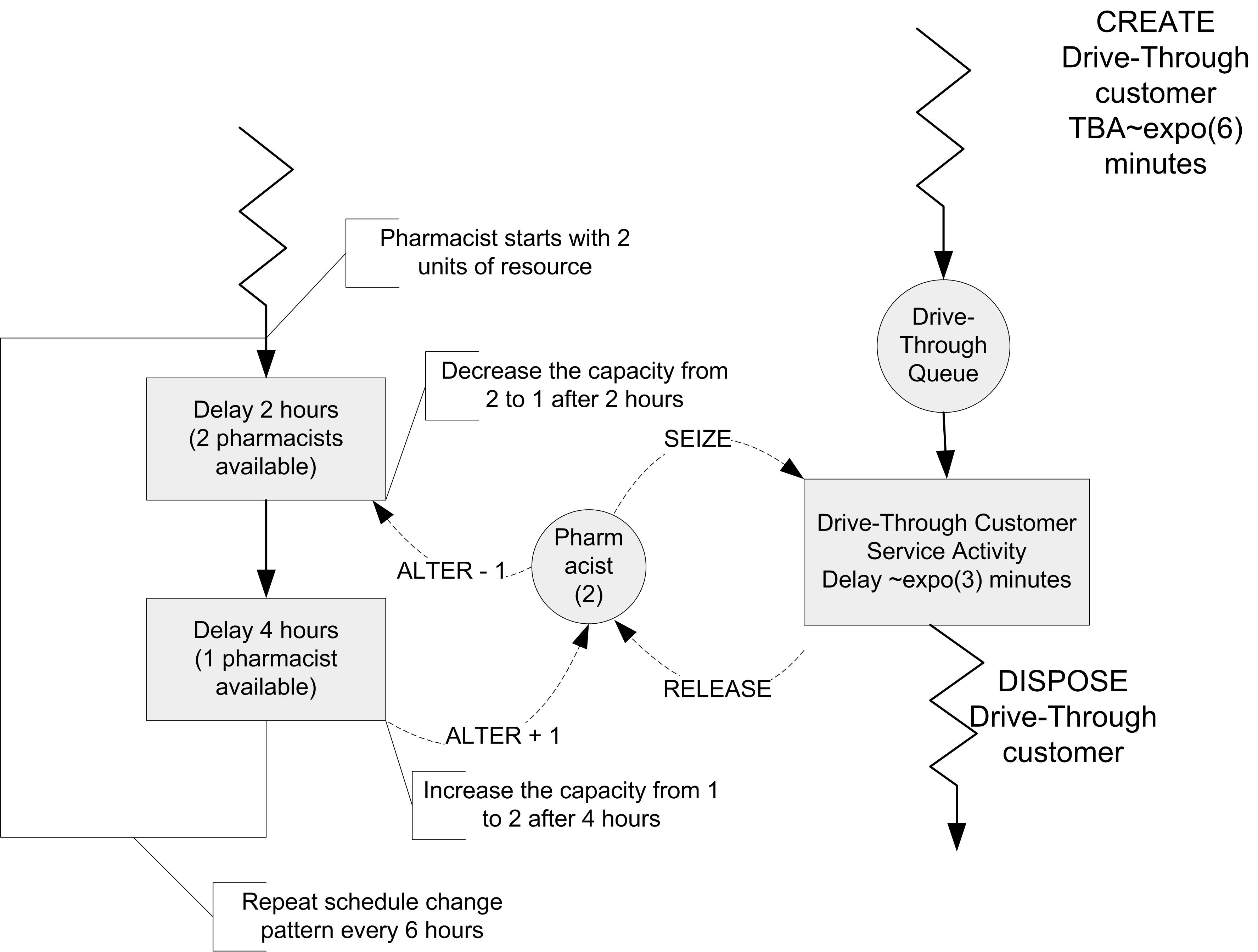
Figure 6.5: Activity diagram for scheduled capacity Changes
As an example, consider the following illustration of the SCHEDULE module based on a modified version of Smarts139-ResourceScheduleExample.doe, an SMART file. In this system, customers arrive according to a Poisson process with a rate of 1 customer per minute. The service times of the customers are distributed according to a triangular distribution with parameters (3, 4, 5) in minutes. Each arriving customer requires 1 unit of a single resource when receiving service; however, the capacity of the resource varies with time. Let’s suppose that two, 480 minute shifts, of operation will be simulated. Assuming that the first shift starts at time zero, each shift is staffed with the same pattern, which varies according to the values shown in Table 6.3. With this information, you can easily setup the resource in to follow the staffing plan for the two shifts. This is done by first defining the schedule using the SCHEDULE module and then indicating that the resource should follow the schedule within the appropriate RESOURCE module.
| Shift | Start time | Stop time | # Available | Duration |
|---|---|---|---|---|
| 1 | 0 | 60 | 2 | 60 |
| 1 | 60 | 180 | 3 | 120 |
| 1 | 180 | 360 | 9 | 180 |
| 1 | 360 | 480 | 6 | 120 |
| 2 | 480 | 540 | 2 | 60 |
| 2 | 540 | 660 | 3 | 120 |
| 2 | 660 | 840 | 9 | 180 |
| 2 | 840 | 960 | 6 | 120 |
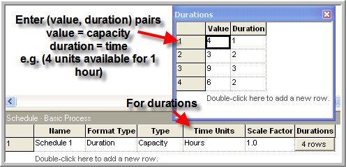
Figure 6.6: Resource schedule value, duration data sheet view
To setup the schedule, there are a number of schedule editing formats available. Figure 6.6 shows the schedule spreadsheet editor for this example. In the data sheet, you can enter (value, duration) pairs that represent the capacity and the duration of time that the capacity will be available. The schedule must be given a name, format type (Duration), type (Capacity for resources), and time units (hours in this case). The scale factor field does not apply to capacity type schedules.
The Schedule dialog box is also useful in entering a schedule. The method of schedule editing is entirely your preference. Arena also allows schedules to be read in from Excel.
In the SCHEDULE module, only the schedule for the first 480 minute shift was entered. What happens when the duration specified by the schedule are completed? The default action is to repeat the schedule indefinitely until the simulation run length is completed. If you want a specific capacity to remain for entire run you can enter a blank duration. This defaults the duration to infinite. The schedule will not repeat so that the capacity will remain at the specified value when the duration is invoked.
Once the schedule has been defined, you need to specify that the resource will follow the schedule by changing its Type to "Based on Schedule" as shown in Figure 6.7. In addition, you must specify the rule that the resource will use if there is a schedule change and it is currently seized by entities. This is called the Schedule Rule. There are three rules available:
- Ignore
starts the time duration of the schedule change or failure immediately, but allows the busy resource to finish processing the current entity before effecting the capacity change.
- Wait
waits until the busy resource has finished processing the current entity before changing the resource capacity or starting the failure and starting the time duration of the schedule change/failure.
- Preempt
interrupts the currently-processing entity, changes the resource capacity and starts the time duration of the schedule change or failure immediately. The resource will resume processing the preempted entity as soon as the resource becomes available (after schedule change/failure).
The wait rule has been used in Figure 6.7. Let’s discuss a bit more on how these rules function with an example.
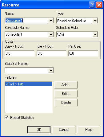
Figure 6.7: RESOURCE module dialog with schedule capacity
Let’s suppose that your simulation professor has office hours throughout the day, except from 12-12:30 pm for lunch. In addition, since your professor teaches simulation using , he or she follows Arena’s rules for capacity changes. What happens for each rule if you arrive at 11:55 am with a question?
Ignore Case 1:
You arrive at 11:55 am with a 10 minute question and begin service.
At Noon, the professor gets up and hangs a Lunch in Progress sign.
Your professor continues to answer your question for the remaining service time of 5 minutes.
You leave at 12:05 pm.
Whether or not there are any students waiting in the hallway, the professor still starts lunch.
At 12:30 pm the professor finishes lunch and takes down the lunch in progress sign. If there were any students waiting in the hallway, they can begin service.
The net effect of case 1 is that the professor lost 5 minutes of lunch time. During the 30 minute schedule break, the professor was busy for 5 minutes and inactive for 25 minutes.
Ignore Case 2:
You arrive at 11:55 am with a 45 minute question and begin service.
At Noon, the professor gets up and hangs a Lunch in Progress sign.
Your professor continues to answer your question for the remaining service time of 40 minutes.
At 12:30 pm the professor gets up and takes down the lunch in progress sign and continues to answer your question.
You leave at 12:40 pm
The net effect of case 2 is that the professor did not get to eat lunch that day. During the 30 minute scheduled break, the professor was busy for 30 minutes.
This rule is called Ignore since the scheduled break may be ignored by the resource if the resource is busy when the break occurs. Technically, the scheduled break actually occurs and the time that was scheduled is considered as unscheduled (inactive) time.
Let’s assume that the professor is at work for 8 hours each day (including the lunch break). But because of the scheduled lunch break, the total time available for useful work is 450 minutes. In case 1, the professor worked for 5 minutes more than they were scheduled. In case 2, the professor worked for 30 minutes more than they were scheduled. As will be indicated shortly, this extra work time, must be factored into how the utilization of the resource (professor) is computed. Now, let’s examine what happens if the rule is Wait.
Wait Case 1:
You arrive at 11:55 am with a 10 minute question and begin service.
At Noon, the professor’s lunch reminder rings on his or her computer. The professor recognizes the reminder but doesn’t act on it, yet.
Your professor continues to answer your question for the remaining service time of 5 minutes.
You leave at 12:05 pm. The professor recalls the lunch reminder and hangs a Lunch in Progress sign. Whether or not there are any students waiting in the hallway, the professor still hangs the sign and starts a 30 minute lunch.
At 12:35 pm the professor finishes lunch and takes down the lunch in progress sign. If there were any students waiting in the hallway, they can begin service.
Wait Case 2:
You arrive at 11:55 am with a 45 minute question and begin service.
At Noon, the professor’s lunch reminder rings on his or her computer. The professor recognizes the reminder but doesn’t act on it, yet.
Your professor continues to answer your question for the remaining service time of 40 minutes.
You leave at 12:40 pm. The professor recalls the lunch reminder and hangs a Lunch in Progress sign. Whether or not there are any students waiting in the hallway, the professor still hangs the sign and starts a 30 minute lunch.
At 1:10 pm the professor finishes lunch and takes down the lunch in progress sign. If there were any students waiting in the hallway, they can begin service.
The net effect of both these cases is that the professor does not miss lunch (unless the student’s question takes the rest of the afternoon !). Thus, in this case the resource will experience the scheduled break after waiting to complete the entity in progress. Again, in this case, the tabulation of the amount of busy time may be affected by when the rule is invoked. Now, let’s consider the situation of the Preempt rule.
Preempt Case 1:
You arrive at 11:55 am with a 10 minute question and begin service.
At Noon, the professor’s lunch reminder rings on his or her computer. The professor gets up, pushes you into the corner of the office, hangs the Lunch in Progress sign and begins a 30 minute lunch. If there are any students waiting in the hallway, they continue to wait.
You wait patiently in the corner of the office until 12:30 pm.
At 12:30 pm the professor finishes lunch, takes down the lunch in progress sign, and tells you that you can get out of the corner. You continue your question for the remaining 5 minutes.
At 12:35 pm, you finally finish your 10 minute question and depart the system, wondering what the professor had to eat that was so important.
As you can see from the handling of case 1, the professor always gets the lunch break. The customer’s service is preempted and resumed after the scheduled break. The result for case 2 is essentially the same, with the student finally completing service at 12:55 pm. While this rule may seem a bit rude in a service situation, it is quite reasonable for many situations where the service can be restarted (e.g. parts on a machine).
The example involving the professor involved a resource with 1 unit of capacity. But what happens if the resource has a capacity of more than 1 and what happens if the capacity change is more than 1. The rules work essentially the same. If the scheduled change (decrease) is less than or equal to the current number of idle units, then the rules are not invoked. If the scheduled change will require busy units, then any idle units are first taken away and then the rules are invoked. In the case of the ignore rule, the units continue serving, the inactive sign goes up, and whichever unit is released first becomes inactive first.
Now, that you understand the consequences of the rules, let’s run the example model. The final model including the animation is shown in Figure 6.8. When you run the model, the variable animation boxes will display the current time (in minutes), the current number of scheduled resource units (MR), the current number of busy resource units (NR), and the state of the resource (as per the resource state constants). After running the model for 960 minutes the resource statistics results can be seen in Figure 6.9. Now, you should notice something new. In all prior work, the instantaneous utilization was the same as the scheduled utilization. In this case, these quantities are not the same. The tabulation of the amount of busy time as per the scheduled rules accounts for the difference. Let’s take a more detailed look at how these quantities are computed.
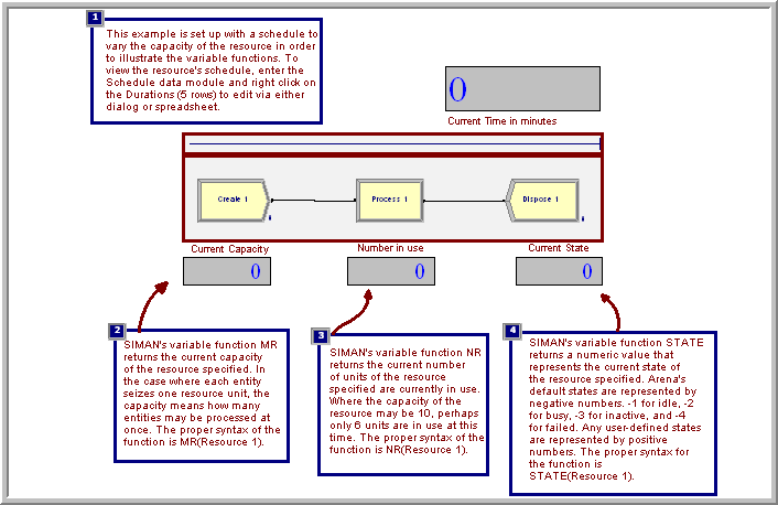
Figure 6.8: Scheduled capacity change model
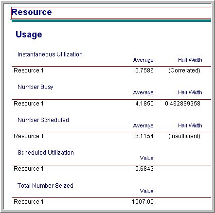
Figure 6.9: Scheduled capacity change model results
6.2.2 Calculating Utilization
The calculation of instantaneous and scheduled utilization depends upon the two variables \(\mathit{NR}\) and \(\mathit{MR}\) for a resource. The instantaneous utilization is defined as the time weighted average of the ratio of these variables. Let \(\mathit{NR}(t)\) be the number of busy resource units at time \(t\). Then, the time average number of busy resources is:
\[\overline{\mathit{NR}} = \frac{1}{T}\int\limits_0^T \mathit{NR}(t) \mathrm{d}t\]
Let \(\mathit{MR}(t)\) be the number of scheduled resource units at time \(t\). Then, the time average number of scheduled resource units is:
\[\overline{\mathit{MR}} = \frac{1}{T}\int\limits_0^T \mathit{MR}(t) \mathrm{d}t\]
Now, we can define the instantaneous utilization at time \(t\) as:
\[IU(t) = \begin{cases} 0 & \mathit{NR}(t) = 0\\ 1 & \mathit{NR}(t) \geq \mathit{MR}(t)\\ \mathit{NR}(t)/\mathit{MR}(t) & \text{otherwise} \end{cases}\]
Thus, the time average instantaneous utilization is:
\[\overline{\mathit{IU}} = \frac{1}{T}\int\limits_0^T \mathit{IU}(t)\mathrm{d}t\]
The scheduled utilization is the time average number of busy resources divided by the time average number scheduled. As can be seen in Equation (6.1), this is the same as the total time spent busy divided by the total time available for all resource units.
\[\begin{equation} \overline{\mathit{SU}} = \frac{\overline{\mathit{NR}}}{\overline{\mathit{MR}}} = \frac{\frac{1}{T}\int\limits_0^T \mathit{NR}(t)dt}{\frac{1}{T}\int\limits_0^T \mathit{MR}(t)dt} = \frac{\int\limits_0^T \mathit{NR}(t)dt}{\int\limits_0^T \mathit{MR}(t)dt} \tag{6.1} \end{equation}\]
If \(\mathit{MR}(t)\) is constant, then \(\overline{\mathit{IU}} = \overline{\mathit{SU}}\). The function, RESUTIL(Resource ID) returns \(\mathit{IU}(t)\). Caution should be used in interpreting \(\overline{\mathit{IU}}\) when \(\mathit{MR}(t)\) varies with time.
Now let’s return to the example of the professor holding office hours. Let’s suppose that the ignore option is used and consider case 2 and the 45 minute question. Let’s also assume for simplicity that the professor had a take home exam due the next day and was therefore busy all day long. What would be the average instantaneous utilization and the scheduled utilization of the professor? Table 6.4 illustrates the calculations.
| Time interval | Busy time | Scheduled time | \(\mathit{NR}(t)\) | \(\mathit{MR}(t)\) | \(\mathit{IU}(t)\) |
|---|---|---|---|---|---|
| 8 am - noon | 240 | 240 | 1.0 | 1.0 | 1.0 |
| 12 - 12:30 pm | 30 | 0 | 1.0 | 0 | 1.0 |
| 12:30 - 4 pm | 210 | 210 | 1.0 | 1.0 | 1.0 |
| 480 | 450 |
From Table 6.4 we can compute \(\overline{\mathit{NR}}\) and \(\overline{\mathit{MR}}\) as:
\[\begin{aligned} \overline{\mathit{NR}} & = \frac{1}{480}\int\limits_{0}^{480} 1.0 \mathrm{d}t = \frac{480}{480} = 1.0 \\ \overline{\mathit{MR}} & = \frac{1}{480}\int\limits_{0}^{480} \mathit{MR(t)} \mathrm{d}t = \frac{1}{480}\biggl\lbrace\int\limits_{0}^{240} 1.0 \mathrm{d}t + \int\limits_{270}^{480} 1.0 \mathrm{d}t \biggr\rbrace = 450/480 = 0.9375\\ \overline{\mathit{IU}} & = \frac{1}{480}\int\limits_{0}^{480} 1.0 \mathrm{d}t = \frac{480}{480} = 1.0\\ \overline{\mathit{SU}} & = \frac{\overline{\mathit{NR}}}{\overline{\mathit{MR}}} = \frac{1.0}{0.9375} = 1.0\bar{6}\end{aligned}\]
Table 6.4 indicates that \(\overline{IU}\) = 1.0 (or 100%) and \(\overline{SU}\) = 1.06 (or 106%). Who says that professors don’t give their all! Thus, with scheduled utilization, a schedule can result in the resource having its scheduled utilization higher than 100%. There is nothing wrong with this result, and if it is the case that the resource is busy for more time than it is scheduled, you would definitely want to know.
The help system has an excellent discussion of how it calculates instantaneous and scheduled utilization (as well as what they mean) in its help files, see Figure 6.10. The interested read should search under, resource statistics: Instantaneous Utilization Vs. Scheduled utilization.
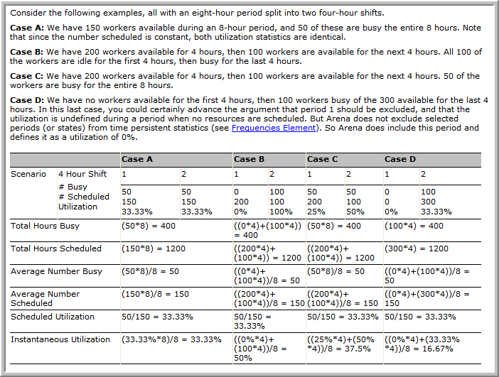
Figure 6.10: Utilization example from Help files
6.2.3 Resource Failure Modeling
As mentioned, a resource has 4 states that it can be in: idle, busy, inactive, and failed. The SCHEDULE module is used to model planned capacity changes. The FAILURES module is used to model unplanned or random capacity changes that place the resource in the failed state. The failed state represents the situation of a breakdown for the entire resource. When a failure occurs for a resource, all units of the resource become unavailable and the resource is placed in the failed state. For example, imagine standing in line at a bank with 3 tellers. For some reason, the computer system goes down and all tellers are thus unable to perform work. This situation is modeled with the FAILURES module of the Advanced Process panel. A more common application of failure modeling occurs in manufacturing settings to model the failure and repair of production equipment.
There are two ways in which a failure can be initiated for a resource: time based and usage (count) based. The concept of time based failures is illustrated in Figure 6.11. Notice the similarity to scheduled capacity changes. You can think of this situation as a failure "clock" ticking. The up-time delay is governed by the time to failure distribution and the downtime delay is governed by the time to repair distribution. When the time of failure occurs, the resource is placed in the failed state. If the resource has busy units, then the rules for capacity change (ignore, wait, and preempt) are invoked.
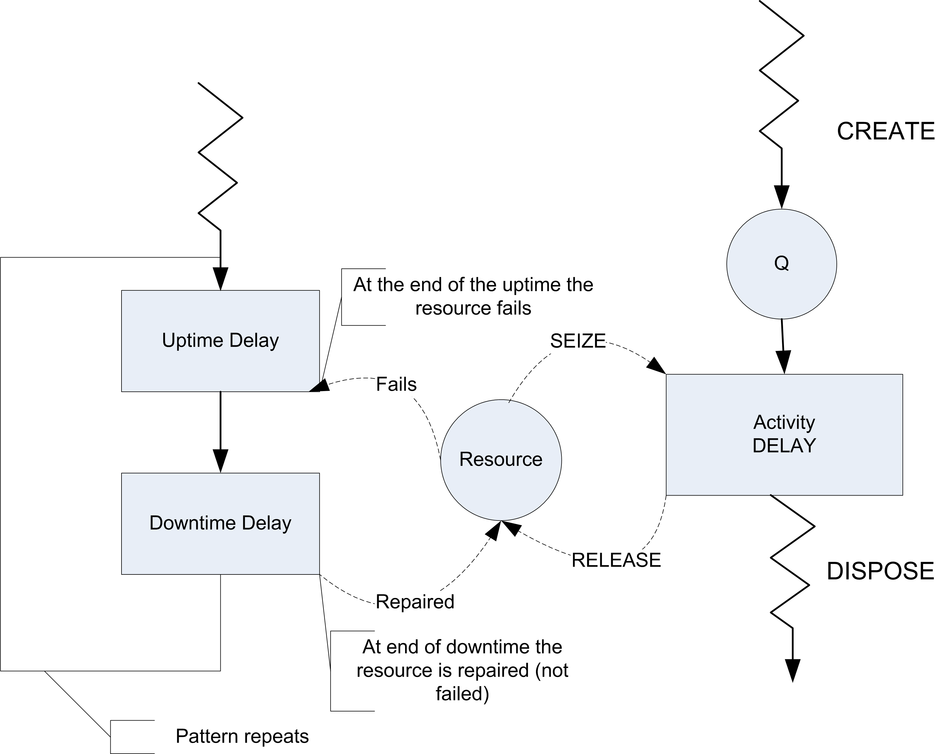
Figure 6.11: Activity diagram for failure modeling
Usage based failures occur after the resource has been released. Each time the resource is released a count is incremented, when it reaches the specified number until failure value, the resource fails. Again, if the resource has busy units the capacity change rules are invoked. A resource can have multiple failures (both time and count based) defined to govern its behavior. In the case of multiple failures that occur before the repair, the failures queue up and cause the repair times to be acted on consecutively.
Figure 6.12 and Figure 6.13 illustrate how to define count based and time based failures within the FAILURES module.
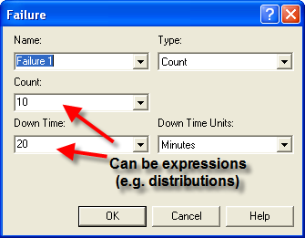
Figure 6.12: Count cased failure dialog
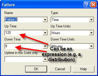
Figure 6.13: Time based failure dialog
In both cases, the up-time, downtime, or count fields can all be expressions. In the case of the time based failure (Figure 6.13) the field up-time in this State only requires special mention. A time based failure defines a failure event that is scheduled to occur when the failure occurs. After the failure is repaired, the event is re-scheduled and the time to failure starts again. The up-time in this state field forms the basis for the time to failure. If nothing is specified, then simulation clock time is used as the basis. However, you can specify a state (from a STATESET or auto state (Idle, Busy, etc)) to use as the basis for accumulating the time until failure. The most common situation is to choose the Busy state. In this fashion, the resource only accumulates time until failure during its busy time. Figure 6.14 and Figure 6.15 illustrate how to attach the failures to resources.
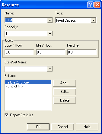
Figure 6.14: Resource with failure attached
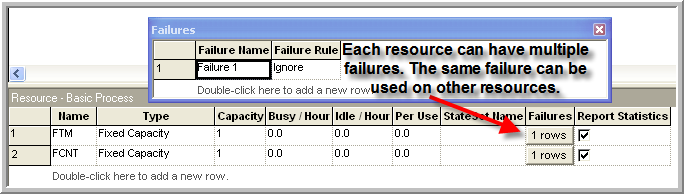
Figure 6.15: Resource with failures data sheet view
Notice that in the case of Figure 6.15}, you can clearly see that a resource can have multiple failures. In addition, the same failure can be attached to different resources. These figures are all based on the file, Smarts112-TimeAndCountFailures.doe, which accompanies this chapter. In this file, resource animation is used to indicate that the resource is in the failed state. You are encouraged to run the model. You might also look at the Smarts123.doe file for other ideas about displaying failures.
The next section illustrates how to use resource scheduled capacity changes to effectively model a system with non-stationary arrivals.