2.12 Exercises
The \(\underline{\hspace{3cm}}\) of a system is defined to be that collection of variables necessary to describe the system at any time, relative to the objectives of study.
An \(\underline{\hspace{3cm}}\) is defined as an instantaneous occurrence that may change the state of the system.
An \(\underline{\hspace{3cm}}\) describes the properties of entities by data values.
| Concept | Definition |
|---|---|
| (a) | Represented as a circle with a queue name labeled inside |
| (b) | Shown as a rectangle with an appropriate label inside |
| Resource | (c) |
| Lines/arcs | (d) |
| (e) | Indicates the creation or destruction of an entity |
Exercise 2.8 Develop a model to generate 30 observations from the following probability density function:
\[ f(x) = \begin{cases} \dfrac{3x^2}{2} & -1 \leq x \leq 1\\ 0 & \text{otherwise} \\ \end{cases} \] Report the minimum, maximum, sample average, and 95% confidence interval half-width of the observations.Exercise 2.9 Suppose that the service time for a patient consists of two distributions. There is a 25% chance that the service time is uniformly distributed with minimum of 20 minutes and a maximum of 25 minutes, and a 75% chance that the time is distributed according to a Weibull distribution with shape of 2 and a scale of 4.5.
Setup a model to generate 100 observations of the service time. Compute the theoretical expected value of the distribution. Estimate the expected value of the distribution and compute a 95% confidence interval on the expected value. Did your confidence interval contain the theoretical expected value of the distribution?Exercise 2.10 Suppose that \(X\) is a random variable with a \(N(\mu = 2, \sigma = 1.5)\) normal distribution. Generate 100 observations of \(X\) using a simulation model.
Estimate the mean from your observations. Report a 95% confidence interval for your point estimate.
Estimate the variance from your observations. Report a 95% confidence interval for your point estimate.
Estimate the \(P(X>3)\) from your observations. Report a 95% confidence interval for your point estimate.| \(x\) | 0 | 1 | 2 | 3 | 4 |
|---|---|---|---|---|---|
| \(p(x)\) | 0.3 | 0.2 | 0.2 | 0.1 | 0.2 |
| Demand | 0 | 1 | 2 |
|---|---|---|---|
| Probability | 0.3 | 0.2 | 0.5 |
Exercise 2.14 Using and the Monte Carlo method estimate the following integral with 95% confidence to within \(\pm 0.01\).
\[\int\limits_{1}^{4} \left( \sqrt{x} + \frac{1}{2\sqrt{x}}\right) \mathrm{d}x\]Exercise 2.15 Using and the Monte Carlo method estimate the following integral with 99% confidence to within \(\pm 0.01\).
\[\int\limits_{0}^{\pi} \left( \sin (x) - 8x^{2}\right) \mathrm{d}x\]
Exercise 2.16 Using and the Monte Carlo method estimate the following integral with 99% confidence to within \(\pm 0.01\).
\[\theta = \int\limits_{0}^{1} \int\limits_{0}^{1} \left( 4x^{2}y + y^{2}\right) \mathrm{d}x \mathrm{d}y\]
| years | 4 | 5 | 6 | 7 |
|---|---|---|---|---|
| f(years) | 0.3 | 0.4 | 0.1 | 0.2 |
| F(years) | 0.3 | 0.7 | 0.8 | 1.0 |
The interest rate has been varying recently and the firm is unsure of the rate for performing the analysis. To be safe, they have decided that the interest rate should be modeled as a beta random variable over the range from 6 to 9 percent with alpha = 5.0 and beta = 1.5. Given all the uncertain elements in the situation, they have decided to perform a simulation analysis in order to assess the expected present value of the decision and the chance that the decision has a negative return.
We desire to be 95% confident that our estimate of the true expected present value is within \(\pm\) 10 dollars. Develop a model for this situation.
| End of Year | 0 | 1 | 2 | 3 | 4 |
|---|---|---|---|---|---|
| A | \(N(-250, 10)\) | \(N(75, 10)\) | \(N(75, 10)\) | \(N(175, 20)\) | \(N(150, 40)\) |
| B | \(N(-250, 5)\) | \(N(150, 10)\) | \(N(150, 10)\) | \(N(75, 20)\) | \(N(75, 30)\) |
The interest rate has been varying recently and the firm is unsure of the rate for performing the analysis. To be safe, they have decided that the interest rate should be modeled as a beta random variable over the range from 2 to 7 percent with \(\alpha_1 = 4.0\) and \(\alpha_2 = 1.2\). Given all the uncertain elements in the situation, they have decided to perform a simulation analysis in order to assess the situation. Use to answer the following questions:
Compare the expected present worth of the two alternatives. Estimate the probability that alternative A has a higher present worth than alternative B.
Determine the number of samples needed to be 95% confidence that you have estimated the \(P[PW(A) > PW(B)]\) to within \(\pm\) 0.10.
Exercise 2.19 A U-shaped component is to be formed from the three parts A, B, and C. The picture is shown in the figure below. The length of A is lognormally distributed with a mean of 20 millimeters and a standard deviation of 0.2 millimeter. The thickness of parts B and C is uniformly distributed with a minimum of 4.98 millimeters and a maximum of 5.02 millimeters. Assume all dimensions are independent.
Develop a model to estimate the probability that the gap \(D\) is less than 10.1 millimeters with 95% confidence to within plus or minus 0.01.
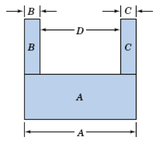
Figure 2.74: U-Shaped Component
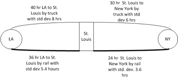
Figure 2.75: Truck Paths
Assume that the travel times (in either direction) are lognormally distributed as shown in the figure. For example, the time from NY to St. Louis (or St. Louis to NY) by truck is 30 hours with a standard deviation of 6 hours. In addition, assume that the transfer time in hours in St. Louis is triangularly distributed with parameters (8, 10, 12) for trucks (truck to truck). The transfer time in hours involving rail is triangularly distributed with parameters (13, 15, 17) for rail (rail to rail, rail to truck, truck to rail). We are interested in determining the shortest total shipment time combination from NY to LA. Develop an simulation for this problem.
How many shipment combinations are there?
Write an expression for the total shipment time of the truck only combination.
We are interested in estimating the average shipment time for each shipment combination and the probability that the shipment combination will be able to deliver the shipment within 85 hours.
Estimate the probability that a shipping combination will be the shortest.
Exercise 2.21 A firm produces YBox gaming stations for the consumer market. Their profit function is: \[\text{Profit} = (\text{unit price} - \text{unit cost})\times(\text{quantity sold}) - \text{fixed costs}\]
Suppose that the unit price is $200 per gaming station, and that the other variables have the following probability distributions:| Unit Cost | 80 | 90 | 100 | 110 |
|---|---|---|---|---|
| Probability | 0.20 | 0.40 | 0.30 | 0.10 |
| Quantity Sold | 1000 | 2000 | 3000 | |
| Probability | 0.10 | 0.60 | 0.30 | |
| Fixed Cost | 50000 | 65000 | 80000 | |
| Probability | 0.40 | 0.30 | 0.30 |
Use a simulation model to generate 1000 observations of the profit.
Estimate the mean profit from your sample and compute a 95% confidence interval for the mean profit. Estimate the probability that the profit will be positive.
Exercise 2.22 T. Wilson operates a sports magazine stand before each game. He can buy each magazine for 33 cents and can sell each magazine for 50 cents. Magazines not sold at the end of the game are sold for scrap for 5 cents each. Magazines can only be purchased in bundles of 10. Thus, he can buy 10, 20, and so on magazines prior to the game to stock his stand. The lost revenue for not meeting demand is 17 cents for each magazine demanded that could not be provided. Mr. Wilson’s profit is as follows:
\[\begin{aligned} \text{Profit} & = (\text{revenue from sales}) - (\text{cost of magazines}) \\ & - (\text{lost profit from excess demand}) \\ & + (\text{salvage value from sale of scrap magazines}) \end{aligned} \]
Not all game days are the same in terms of potential demand. The type of day depends on a number of factors including the current standings, the opponent, and whether or not there are other special events planned for the game day weekend. There are three types of game days demand: high, medium, low. The type of day has a probability distribution associated with it.
| Type of Day | High | Medium | Low |
|---|---|---|---|
| Probability | 0.35 | 0.45 | 0.20 |
The amount of demand for magazines then depends on the type of day according to the following distributions:
| Demand | PMF | CDF | PMF | CDF | PMF | CDF |
| 40 | 0.03 | 0.03 | 0.1 | 0.1 | 0.44 | 0.44 |
| 50 | 0.05 | 0.08 | 0.18 | 0.28 | 0.22 | 0.66 |
| 60 | 0.15 | 0.23 | 0.4 | 0.68 | 0.16 | 0.82 |
| 70 | 0.2 | 0.43 | 0.2 | 0.88 | 0.12 | 0.94 |
| 80 | 0.35 | 0.78 | 0.08 | 0.96 | 0.06 | 1.0 |
| 90 | 0.15 | 0.93 | 0.04 | 1.0 | ||
| 100 | 0.07 | 1.0 |
Let \(Q\) be the number of units of magazines purchased (quantity on hand) to setup the stand. Let \(D\) represent the demand for the game day. If \(D > Q\), Mr. Wilson sells only \(Q\) and will have lost sales of \(D-Q\). If \(D < Q\), Mr. Wilson sells only \(D\) and will have scrap of \(Q-D\). Assume that he has determined that \(Q = 50\).
Make sure that you can estimate the average profit and the probability that the profit is greater than zero for Mr. Wilson. Develop a model to estimate the average profit based on 100 observations.
Exercise 2.23 The time for an automated storage and retrieval system in a warehouse to locate a part consists of three movements. Let \(X\) be the time to travel to the correct aisle. Let \(Y\) be the time to travel to the correct location along the aisle. And let \(Z\) be the time to travel up to the correct location on the shelves. Assume that the distributions of \(X\), \(Y\), and \(Z\) are as follows:
\(X \sim\) lognormal with mean 20 and standard deviation 10 seconds
\(Y \sim\) uniform with minimum 10 and maximum 15 seconds
\(Z \sim\) uniform with minimum of 5 and a maximum of 10 seconds
Develop a model that can estimate the average total time that it takes to locate a part and can estimate the probability that the time to locate a part exceeds 60 seconds. Base your analysis on 1000 observations.
| Daily Demand (items) | 4 | 5 | 6 | 7 | 8 |
|---|---|---|---|---|---|
| Probability | 0.10 | 0.30 | 0.35 | 0.10 | 0.15 |
The lead-time is the number of days from placing an order until the firm receives the order from the supplier.
Assume that the lead-time is a constant 10 days. Develop a model to simulate 1000 instances of LDT. Report the summary statistics for the 1000 observations. Estimate the chance that LDT is greater than or equal to 10. Report a 95% confidence interval on your estimate.
Assume that the lead-time has a shifted geometric distribution with probability parameter equal to 0.2 Use a model to simulate 1000 instances of LDT. Report the summary statistics for the 1000 observations. Estimate the chance that LDT is greater than or equal to 10. Report a 95% confidence interval on your estimate.
Exercise 2.25 If \(Z \sim N(0,1)\), and \(Y = \sum_{i=1}^k Z_i^2\) then \(Y \sim \chi_k^2\), where \(\chi_k^2\) is a chi-squared random variable with \(k\) degrees of freedom. Setup a model to generate 50 \(\chi_5^2\) random variates. Report the minimum, maximum, sample average, and 95% confidence interval half-width of the observations.
Exercise 2.26 Setup a model that will generate 30 observations from the following probability density function using the Acceptance-Rejection algorithm for generating random variates.
\[f(x) = \begin{cases} \dfrac{3x^2}{2} & -1 \leq x \leq 1\\ 0 & \text{otherwise} \\ \end{cases}\]
Exercise 2.27 This procedure is due to (Box and Muller 1958). Let \(U_1\) and \(U_2\) be two independent uniform (0,1) random variables and define:
\[\begin{aligned} X_1 & = \cos (2 \pi U_2) \sqrt{-2 ln(U_1)}\\ X_2 & = \sin (2 \pi U_2) \sqrt{-2 ln(U_1)}\end{aligned}\]
It can be shown that \(X_1\) and \(X_2\) will be independent standard normal random variables, i.e. \(N(0,1)\). Use to implement the Box and Muller algorithm for generating normal random variables. Generate 1000 \(N(\mu = 2, \sigma = 0.75)\) random variables via this method. Report the minimum, maximum, sample average, and 95% confidence interval half-width of the observations.
Exercise 2.28 Using the supplied data set, draw the sample path for the state variable, \(Y(t)\). Assume that the value of \(Y(t)\) is the value of the state variable just after time \(t\). Compute the time average over the supplied time range.
| \(t\) | 0 | 1 | 6 | 10 | 15 | 18 | 20 | 25 | 30 | 34 | 39 | 42 |
| \(Y(t)\) | 1 | 2 | 1 | 1 | 1 | 2 | 2 | 3 | 2 | 1 | 0 | 1 |
Exercise 2.29 Using the supplied data set, draw the sample path for the state variable, \(N(t)\). Give a formula for estimating the time average number in the system, \(N(t)\), and then use the data to compute the time average number in the system over the range from 0 to 25. Assume that the value of \(N(t\) is the value of the state variable just after time \(t\).
| \(t\) | 0 | 2 | 4 | 5 | 7 | 10 | 12 | 15 | 20 |
| \(N(t)\) | 0 | 1 | 0 | 1 | 2 | 3 | 2 | 1 | 0 |
| Customer | Time of | Service |
| Number | Arrival | Time |
| 1 | 3 | 4 |
| 2 | 11 | 4 |
| 3 | 13 | 4 |
| 4 | 14 | 3 |
| 5 | 17 | 2 |
| 6 | 19 | 4 |
| 7 | 21 | 3 |
| 8 | 27 | 2 |
| 9 | 32 | 2 |
| 10 | 35 | 4 |
| 11 | 38 | 3 |
| 12 | 45 | 2 |
| 13 | 50 | 3 |
| 14 | 53 | 4 |
| 15 | 55 | 4 |
Complete a table similar to that used in the chapter and compute the average of the system times for the customers. What percentage of the total time was the teller idle? Compute the percentage of time that there were 0, 1, 2, and 3 customers in the queue.
| Customer | Inter-Arrival | Service | Time of |
| Number | Time | Time | Arrival |
| 1 | 22 | 74 | 22 |
| 2 | 89 | 105 | 111 |
| 3 | 21 | 34 | 132 |
| 4 | 26 | 38 | 158 |
| 5 | 80 | 23 | |
| 6 | 81 | 26 | |
| 7 | 78 | 90 | |
| 8 | 20 | 26 | |
| 9 | 32 | 37 | |
| 10 | 13 | 88 | |
| 11 | 28 | 38 | |
| 12 | 18 | 73 | |
| 13 | 29 | 93 | |
| 14 | 19 | 25 | |
| 15 | 20 | 93 | |
| 16 | 23 | 5 | |
| 17 | 78 | 37 | |
| 18 | 20 | 51 | |
| 19 | 109 | 28 | |
| 20 | 78 | 85 |
We are given the inter-arrival times. Determine the time of arrival of each customer. Complete the event and state variable change table associated with this situation. Draw a sample path graph for the variable \(N(t)\) which represents the number of customers in the system at any time \(t\). Compute the average number of customers in the system over the time period from 0 to 700. Draw a sample path graph for the variable \(NQ(t)\) which represents the number of customers waiting for the server at any time \(t\). Compute the average number of customers in the queue over the time period from 0 to 700. Draw a sample path graph for the variable \(B(t)\) which represents the number of servers busy at any time t. Compute the average number of busy servers in the system over the time period from 0 to 700. Compute the average time spent in the system for the customers.
Exercise 2.32 Parts arrive at a station with a single machine according to a Poisson process with the rate of 1.5 per minute. The time it takes to process the part has an exponential distribution with a mean of 30 second. There is no upper limit on the number of parts that wait for process. Setup an model to estimate the expected number of parts waiting in the queue and the utilization of the machine. Run your model for 10000 seconds for 30 replications and report the results. Use M/M/1 queueing results from the chatper to verify that your simulation is working as intended.
Exercise 2.33 A large car dealer has a policy of providing cars for its customers that have car problems. When a customer brings the car in for repair, that customer has use of a dealer’s car. The dealer estimates that the dealer cost for providing the service is $10 per day for as long as the customer’s car is in the shop. Thus, if the customer’s car was in the shop for 1.5 days, the dealer’s cost would be $15. Arrivals to the shop of customers with car problems form a Poisson process with a mean rate of one every other day. There is one mechanic dedicated to the customer’s car. The time that the mechanic spends on a car can be described by an exponential distribution with a mean of 1.6 days. Setup a model to estimate the expected time within the shop for the cars and the utilization of the mechanic. Run your model for 10000 days for 30 replications and report the results. Estimate the total cost per day to the dealer for this policy. Use the M/M/1 queueing results from the chapter to verify that your simulation is working as intended.
Exercise 2.34 YBox video game players arrive according to a Poisson process with rate 10 per hour to a two-person station for inspection. The inspection time per YBox set is EXPO(10) minutes. On the average 82% of the sets pass inspection. The remaining 18% are routed to an adjustment station with a single operator. Adjustment time per YBox is UNIF(7,14) minutes. After adjustments are made, the units depart the system. The company is interested in the total time spent in the system. Run your model for 10000 minutes for 30 replications and report the results.
Exercise 2.36 The lack of memory property of the exponential distribution states that given \(\Delta t\) is the time period that elapsed since the occurrence of the last event, the time \(t\) remaining until the occurrence of the next event is independent of \(\Delta t\). This implies that, \(P \lbrace X > \Delta t + t|X > t \rbrace = P \lbrace X > t \rbrace\). Describe a simulation experiment that would allow you to test the lack of memory property empirically. Implement your simulation experiment in and test the lack of memory property empirically. Explain in your own words what lack of memory means.
Exercise 2.37 SQL queries arrive to a database server according to a Poisson process with a rate of 1 query every minute. The time that it takes to execute the query on the server is typically between 0.6 and 0.8 minutes uniformly distributed. The server can only execute 1 query at a time. Develop a simulation model to estimate the average delay time for a query