4.5 The LOTR Makers, Inc. Example
In this section, we will develop a model for a small manufacturing system. The purpose of the model is to illustrate how to model with a variety of different distributions, illustrate a common entity creation pattern, and cover the use of resource sets. In a future section we will build on this model in order to compare two system design configurations in a statistically valid manner. We start by introducing the modeling situation. The situation is fictitious but has a number of interesting modeling issues.
Example 4.2 Every morning the sales force at LOTR Makers, Inc. makes a number of confirmation calls to customers who have previously been visited by the sales force. They have tracked the success rate of their confirmation calls over time and have determined that the chance of success varies from day to day. They have modeled the probability of success for a given day as a beta random variable with parameters \(\alpha_1 = 5\) and \(\alpha_2 = 1.5\) so that the mean success rate is about 77%. They always make 100 calls every morning. Each sales call will or will not result in an order for a pair of magical rings for that day. Thus, the number of pairs of rings to produce every day is a binomial random variable, with \(p\) determined by the success rate for the day and \(n = 100\) representing the total number of calls made. Note that \(p\) is random in this modeling.
The sale force is large enough and the time to make the confirmation calls small enough so as to be able to complete all the calls before releasing a production run for the day. In essence, ring production does not start until all the orders have been confirmed, but the actual number of ring pairs produced every day is unknown until the sales call confirmation process is completed. The time to make the calls is negligible when compared to the overall production time.
Besides being magical, one ring is smaller than the other ring so that the smaller ring must fit snuggly inside the larger ring. The pair of rings is produced by a master ring maker and takes uniformly between 5 to 15 minutes. The rings are then scrutinized by an inspector with the time (in minutes) being distributed according to a triangular distribution with parameters (2, 4, 7) for the minimum, the mode, and the maximum. The inspection determines whether the smaller ring is too big or too small when fit inside the bigger outer ring. The inside diameter of the bigger ring, \(D_b\), is normally distributed with a mean of 1.5 cm and a standard deviation of 0.002. The outside diameter of the smaller ring, \(D_s\), is normally distributed with a mean of 1.49 and a standard deviation of 0.005. If \(D_s > D_b\), then the smaller ring will not fit in the bigger ring; however, if \(D_b - D_s > tol\), then the rings are considered too loose. The tolerance is currently set at 0.02 cm.
If there are no problems with the rings, the rings are sent to a packer for custom packaging for shipment. A time study of the packaging time indicates that it is distributed according to a log-normal distribution with a mean of 7 minutes and a standard deviation of 1 minute. If the inspection shows that there is a problem with the pair of rings they are sent to a rework craftsman. The minimum time that it takes to rework the pair of rings has been determined to be 5 minutes plus some random time that is distributed according to a Weibull distribution with a scale parameter of 15 and a shape parameter of 5. After the rework is completed, the pair of rings is sent to packaging.LOTR Makers, Inc. is interested in estimating the daily production time. In particular, management is interested in estimating the probability of overtime. Currently, the company runs two shifts of 480 minutes each. Time after the end of the second shift is considered overtime. Use 30 simulated days to investigate the situation.
4.5.1 Conceptualizing the Model
Now let’s proceed with the modeling of Example 4.2. We start with answering the basic model building questions.
- What is the system? What information is known by the system?
The system is the LOTR Makers, Inc. sales calls and ring production processes. The system starts every day with the initiation of sales calls and ends when the last pair of rings produced for the day is shipped. The system knows the following:
Sales call success probability distribution: \(p \sim BETA(\alpha_1 = 5,\alpha_2 = 1.5)\)
Number of calls to be made every morning: \(n = 100\)
Distribution of time to make the pair of rings:
UNIF(5,15)Distributions associated with the big and small ring diameters:
NORM(1.5, 0.002)andNORM(1.49, 0.005), respectivelyDistribution of ring-inspection time:
TRIA(2,4,7)Distribution of packaging time:
LOGN(7,1)Distribution of rework time,
5 + WEIB(15, 3)Length of a shift: 480 minutes
- What are the entities? What information must be recorded for each entity?
Possible entities are the sales calls and the production job (pair of rings) for every successful sales call. Each sales call knows whether it is successful. For every pair of rings, the diameters must be known.
- What are the resources that are used by the entities?
The sales calls do not use any resources. The production job uses a master craftsman, an inspector, and a packager. It might also use a rework craftsman.
- What are the process flows? Write out or draw sketches of the process.
There are two processes: sales order and production. An outline of the sales order process should look like this:
Start the day.
Determine the likelihood of calls being successful.
Make the calls.
Determine the total number of successful calls.
Start the production jobs.
An outline of the production process should look like this:
Make the rings (determine sizes).
Inspect the rings.
If rings do not pass inspection, perform rework
Package rings and ship.
The next step in the modeling process is to develop pseudo-code for the situation.
Each of the above-described processes needs to be modeled. Note that in the problem statement there is no mention that the sales calls take any significant time. In addition, the sales order process does not use any resources. The calls take place before the production shifts. The major purpose of the sales order process is to determine the number of rings to produce for the daily production run. This type of situation is best modeled using a logical entity. In essence, the logical entity represents the entire sales order process and must determine the number of rings to produce. From the problem statement, this is a binomial random variable with \(n= 100\) and \(p \sim BETA(\alpha_1 = 5,\alpha_2 = 1.5)\). does not have a binomial distribution. The easiest way to accomplish this is to use the convolution property of Bernoulli random variables to generate the binomial random variable.
In the following pseudo-code for the sales order process, the logical entity is first created and then assigned the values of p. Then, 100 Bernoulli random variables are generated to represent the success (or not) of a sales call. The successes are summed so that the appropriate number of production jobs can be determined. In the pseudo-code, the method of summing up the number of successes is done with a looping flow of control construct.
CREATE 1 order process logical entity
BEGIN ASSIGN
 vSalesProb = BETA (5, 1.5)
 myCallNum = 1
END ASSIGN
WHILE myCallNum <= 100
 BEGIGN ASSIGN
    myCallNum = myCallNum + 1
    mySale = DISC(vSalesProb,1,1.0,0)
    myNumSales = myNumSales + mySale
 END ASSIGN
ENDWHILE
SEPARATE
  Original: dispose of original order logical entity
  Duplicate: create myNumSales duplicates, send to LABEL Production
END SEPARATE
The production process pseudo-code describes what happens to a pair of rings as it moves through production.
LABEL: Production
BEGIN PROCESS Ring Making
    SEIZE master ring maker
    DELAY for ring making
    RELEASE master ring maker
END PROCESS
BEGIN ASSIGN
    myIDBigRing = NORM(1.49, 0.005)
    myODSmallRing = NORM(1.5, 0.002)
    myGap = myIDBigRing - myODSmallRing
END ASSIGN
BEGIN PROCESS Inspection
    SEIZE inspector
    DELAY for inspection
    RELEASE inspector
END PROCESS
DECIDE IF myODSmallRing > myIDBigRing
        RECORD too big
        GOTO LABEL: Rework
ELSE
        RECORD not too big
        IF myGap > 0.02
            RECORD too small
            GOTO LABEL: Rework
        ELSE
            RECORD not too small
        ENDIF
END DECIDE
LABEL: Packaging
BEGIN PROCESS Packaging
    SEIZE packager
    DELAY for packaging
    RELEASE packager
END PROCESS
DISPOSE

LABEL: REWORK
BEGIN PROCESS Rework
    SEIZE rework craftsman
    DELAY for rework
    RELEASE rework craftsman
END PROCESS
GOTO LABEL: Packaging
4.5.2 Implementing the Model
Thus far, the system has been conceptualized in terms of entities, resources, and processes. This provides a good understanding of the information that must be represented in the simulation model. In addition, the logical flow of the model has been represented in pseudo-code. Now it is time to implement these ideas. The following describes an implementation for these processes. Before proceeding, you might want to try to implement the logic yourself so that you can check how you are doing against what is presented here. If not, you should try to implement the logic as you proceed through the example.
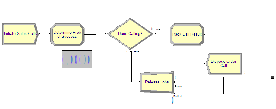
Figure 4.61: Sales confirmation process
To implement the sales order process, you first need to decide how to represent the required data. In the pseudo-code, there is only one entity and no passage of time. In this situation, only 1 entity is needed to execute the associated modules. Thus, either variables or attributes can be used to implement the logic. A variable can be used because there is no danger of another entity changing the global value of the represented variables. In this model, the looping has been implemented using a looping DECIDE construct as discussed in section 4.2. An overview of the sales order portion of the model is given in Figure 4.61. If you are building the model as you follow along, you should take the time to lay down the modules shown in the figure. Each of the modules will be illustrated in what follows.
The CREATE module is very straightforward. Because the Max Arrivals field is 1 and the First Creation field is 0.0, only 1 entity will be created at time 0.0. The fields associated with the label Time between Arrivals are irrelevant in this situation since there will not be any additional arrivals generated from this CREATE module. Fill out your CREATE module as shown in Figure 4.62.
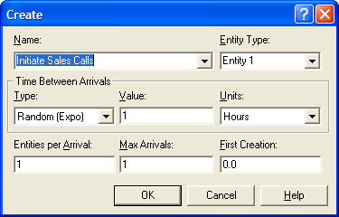
Figure 4.62: Initiating the sales call confirmation process
In the first ASSIGN module, the probability of success for the day is
determined. The variable (vSalesProb) has been used to represent the
probability as drawn from the BETA() distribution function
(Figure 4.63. The attribute (myCallNum) is
initialized to 1, prior to starting the looping logic. This attribute is
going to count the number of calls made.
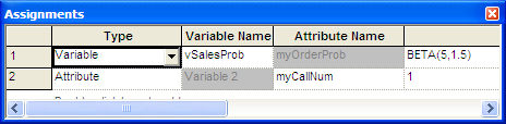
Figure 4.63: Determining the probability of success
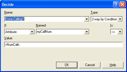
Figure 4.64: Checking that all calls have been made
The DECIDE module in Figure 4.64 uses the attribute (myCallNum) to check the variable vNumCalls. The variable (vNumCalls) is defined
in the VARIABLE module (not shown here) and has been initialized to 100.
Because the total number of calls has been represented as a variable,
the desired number of calls can be easily changed in the VARIABLE
module, without editing the DECIDE module.
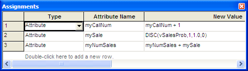
Figure 4.65: Tracking the call results
Figure 4.65 presents the ASSIGN module in the
looping logic. In this ASSIGN, the attribute myCallNum is incremented.
Then, according to the pseudo-code, you must implement a Bernoulli
trial. This can easily be accomplished by using the DISC() distribution
function with only two outcomes, 1 and 0, to assign to the attribute
mySale. You can set the probability of success for the value 1 to
vSalesProb, which was determined via the call to the BETA function.
Note that the function DISC(BETA(5, 1.5), 1, 1.0, 0) would not work in
this situation. DISC(BETA(5, 1.5) will draw a new probability from the
BETA() function every time DISC()is called. Thus, each trial will have
a different probability of success. This is not what is required for the
problem and this is why the variable vSaleProb was determined outside
the looping logic. The attribute (myNumSales) is incremented with the
value from mySale, which essentially counts up all the successful
sales calls (marked with a 1).
When the DECIDE module evaluates to false, all the sales calls have been
made, and the attribute myNumSales has recorded how many successful
calls there have been out of the 100 calls made. The order process
entity is directed to the SEPARATE module where it creates
(myNumSales) duplicates and sends them to the production process
(Figure 4.66. The original order process logic
entity is sent to a DISPOSE, which has its collect entity statistics box
unchecked (not shown). By not checking this box, no statistics will be
collected for entities that exit through this DISPOSE module. Since the
problem does not require anything about the statistics for the order
process logic entity, this is advisable.
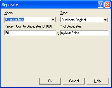
Figure 4.66: Creating the jobs for production
The production process is too long for one screen shot so this discussion is divided into three parts: the making and inspection processes, the decision concerning too big/too small, and the repair and packaging operations. Figure 4.67 presents the making and inspection processes which are implemented with PROCESS modules using the SEIZE, DELAY, RELEASE option. Figure 4.68 and Figure 4.69 show the PROCESS modules and the appropriate delay distributions using the uniform and triangular distributions.
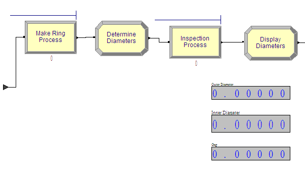
Figure 4.67: Making and inspecting the rings
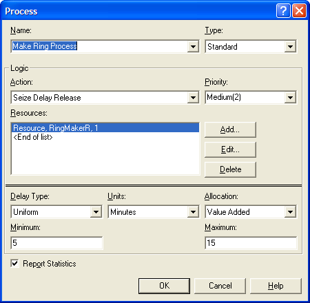
Figure 4.68: PROCESS module for making the rings
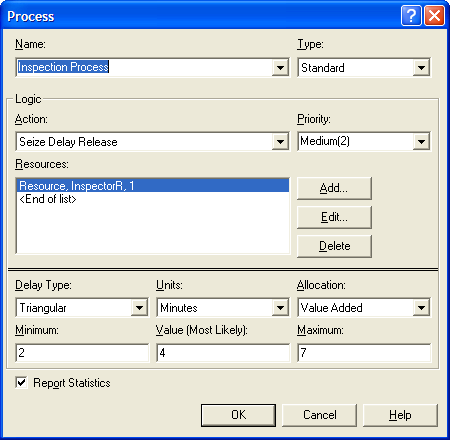
Figure 4.69: PROCESS module for inspecting the rings
The ASSIGN module between the two processes is used to determine the
diameters of the rings.
Figure 4.70 shows that attributes (myIDBigRing
and myODSmallRing) are both set using the normal distribution. The
parameters of the NORM() functions are defined by variables in the
VARIABLE module (not shown here).
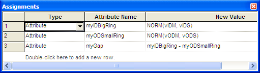
Figure 4.70: Determining the ring diameters
After inspection, the rings must be checked to see whether rework is necessary. An overview of this checking is given in Figure 4.70. The RECORD modules are used to collect statistics on the probability of the smaller ring being too big or the smaller ring being too small.
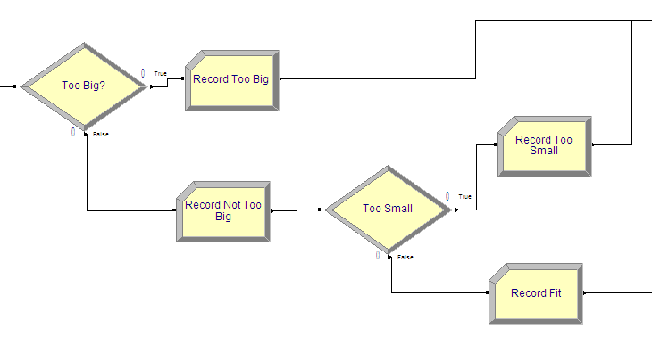
Figure 4.71: Checking ring diameters
Figure 4.72 shows the DECIDE module for
checking if the ring is too big. The 2-way by condition option was used
to check if the attribute (myODSmallRing) is larger than the attribute
(myIDBigRing). If the smaller ring’s outer diameter is larger than the
bigger ring’s inner diameter, then the smaller ring will not fit inside
the bigger ring and the rings will require rework.
Figure4.73 shows the DECIDE module
for checking if the smaller ring is too loose. In this DECIDE module,
the two-way by condition option is used to check the expression
(myIDBigRing - myODSmallRin) > vTol. If the difference between
the diameters of the rings is too large (larger than the tolerance),
then the rings are too loose and need rework. If the rings fit properly,
then they go directly to packaging.
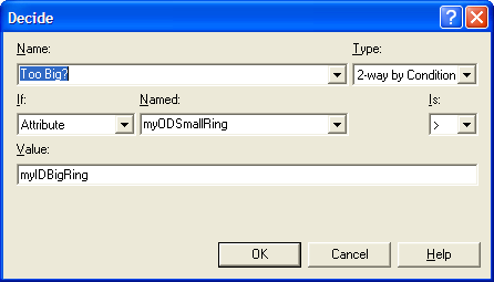
Figure 4.72: Checking to determine whether small ring is too big
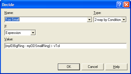
Figure 4.73: Checking to determine whether small ring is too small
Figure 4.74 shows the rework and packaging processes. Again, the PROCESS module is used to represent these processes.
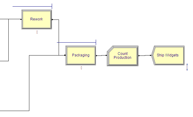
Figure 4.74: Rework and packaging processes
Figures 4.75 and
Figure 4.76 show the rework and packaging
process modules. Note that the delay type has been changed to expression
so that 5 + WEIB(15, 3) and LOGN(7, 1) can be specified for each of the
respective processing times.
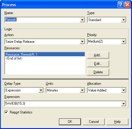
Figure 4.75: Rework PROCESS module
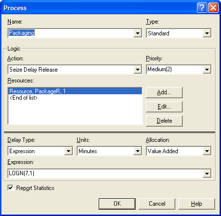
Figure 4.76: Packaging PROCESS module
4.5.3 Running the Model
The completed model for Example 4.2 can be found in the chapter files as LOTRExample.doe. In this section, we will setup and run the model. In Arena, a simulation can end based on three situations:
A scheduled run length
A terminating condition is met
No more events (entities) to process
The problem statement requests the estimation of the probability of overtime work. The sales order process determines the number of rings to produce. The production process continues until there are no more rings to produce for that day. The number of rings to produce is a binomial random variable as determined by the sales order confirmation process. Thus, there is no clear run length for this simulation.
Because the production for the day stops when all the rings are produced, the third situation applies for this model. The simulation will end automatically after all the rings are produced. In essence, a day’s worth of production is simulated. Because the number of rings to produce is random and it takes a random amount of time to make, inspect, rework, and package the rings, the time that the simulation will end is a random variable. If this time is less than 960 (the time of two shifts), there will not be any overtime. If this time is greater than 960, production will have lasted past two shifts and thus overtime will be necessary. To assess the chance that there is overtime, you need to record statistics on how often the end of the simulation is past 960.
Thus, when the simulation ends, TNOW will be the time that the
simulation ended. In this case, TNOW will represent the time that the
last ring completed processing. To estimate the chance that there is
overtime, the Advanced Process Panel’s Statistic module can be used. In
particular, you need to define what is called an OUTPUT statistic.
An OUTPUT statistic records the final value of some system or
statistical value at the end of a replication. An OUTPUT statistic can
be defined by any valid expression involving system variables,
variables, statistical functions, and so on. In
Figure 4.77, an OUTPUT statistic called
TimeToMakeOrderStat has been defined, which records the value of
TNOW. This will cause the collection of statistics (across
replication) for the ending value of TNOW. The OUTPUT statistic will
record the average, minimum, maximum, and half-width across the
replications for the defined expression. You can also use the Output
File field to write out the observed values to a file if necessary.
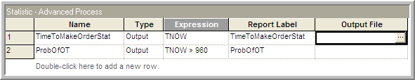
Figure 4.77: Defining OUTPUT statistics for overtime
The second OUTPUT statistic in
Figure 4.77 defines an OUTPUT statistic called
ProbOfOT to represent the chance that the production lasts longer than
960 minutes. In this case, the expression is the Boolean value of
(TNOW > 960). The expression (TNOW > 960) will be evaluated. If
it is true, it will evaluate to 1.0; otherwise, it will evaluate to a
0.0. This is just like an indicator variable on the desired condition.
The OUTPUT statistic will compute the average of the 1’s and 0’s, which
is an estimate of the probability of the condition. Thus, you will get
an estimate of the likelihood of overtime.
Figure 4.78 shows how to set up the run parameters
of the simulation. You should run the simulation with a base time unit
of minutes. This is important to set up here so that TNOW can now be
interpreted in minutes. This ensures that the expression (TNOW > 960) makes sense in terms of the desired units. There is no replication
length specified nor is there a terminating condition specified. As
previously mentioned, the simulation end when there are no more events
(entities) to process. If the model is not set up correctly (i.e., an
infinite number of entities are processed), then the simulation will
never terminate. This is a logical situation that the modeler is
responsible for preventing. The number of replications has been
specified to 30 to represent the 30 days of production.
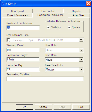
Figure 4.78: Specifying the number of replications in run setup
Running the model results in the user defined statistics for the probability of overtime and the average time to produce the orders as shown in Figure 4.79. The probability of overtime appears to be about 6%, but the 95% half-width is wide for these 30 replications. The average time to produce an order is about 780.68 minutes. While the average is under 960, there still appears to be a reasonable chance of overtime occurring. In the exercises, you are asked to explore the reasons behind the overtime and to recommend an alternative to reduce the likelihood of overtime.
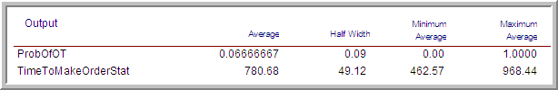
Figure 4.79: LOTR model results across 30 replicated days
In this example, you have learned how to model a small system involving random components and to translate the conceptual model into an simulation. The following explores how independent sampling and common random numbers can be implemented. This example returns to the LOTR Makers system. This example also illustrates the use of resources sets.