2.2 Performing Simple Monte-Carlo Simulations using Arena
The term Monte Carlo generally refers to the set of methods and techniques predicated on estimating quantities by repeatedly sampling from models/equations represented in a computer. As such, this terminology is somewhat synonymous with computer simulation itself. The term Monte Carlo gets its origin from the Monte Carlo casino in the Principality of Monaco, where gambling and games of chance are well known. There is no one Monte Carlo method. Rather there is a collection of algorithms and techniques. In fact, the ideas of random number generation and random variate generation previously discussed form the foundation of Monte Carlo methods.
For the purposes of this chapter, we limit the term Monte Carlo methods to those techniques for generating and estimating the expected values of random variables, especially in regards to static simulation. In static simulation, the notion of time is relatively straightforward with respect to system dynamics. For a static simulation, time ‘ticks’ in a regular pattern and at each ‘tick’ the state of the system changes (new observations are produced). This should be contrasted with dynamic simulation, where the state of the system evolves over time and the state changes at irregularly (randomly occurring) points in time. Dynamic simulation (specifically discrete-event simulation) will be the subject of subsequent sections of this chapter and other chapters in the book.
2.2.1 Simple Monte Carlo Integration
In this section, we will illustrate one of the fundamental uses of Monte Carlo methods: estimating the area of a function. Suppose we have some function, \(g(x)\), defined over the range \(a \leq x \leq b\) and we want to evaluate the integral:
\[\theta = \int\limits_{a}^{b} g(x)\mathrm{d}x\]
Monte Carlo methods allow us to evaluate this integral by couching the problem as an estimation problem. It turns out that the problem can be translated into estimating the expected value of a well-chosen random variable. While a number of different choices for the random variable exist, we will pick one of the simplest for illustrative purposes. Define \(Y\) as follows with \(X \sim U(a,b)\):
\[\begin{equation} Y = \left(b-a\right)g(X) \tag{2.1} \end{equation}\]
Notice that \(Y\) is defined in terms of \(g(X)\), which is also a random variable. Because a function of a random variable is also a random variable, this makes \(Y\) a random variable. Thus, the expectation of \(Y\) can be computed as follows:
\[\begin{equation} E[Y] = E[\left(b-a\right)g(X)] = \left(b-a\right)E[g(X)] \tag{2.2} \end{equation}\]
Now, let us derive, \(E[g(X)]\). By definition,
\[E_{X}[g(X)] = \int\limits_{a}^{b} g(x)f_{X}(x)\mathrm{d}x\]
And, the probability density function for a \(X \sim U(a,b)\) random variable is:
\[f_{X}(x) = \begin{cases} \frac{1}{b-a} & a \leq x \leq b\\ 0 & \text{otherwise} \end{cases}\]
Therefore,
\[E_{X}[g(X)] = \int\limits_{a}^{b} g(x)f_{X}(x)\mathrm{d}x = \int\limits_{a}^{b} g(x)\frac{1}{b-a}\mathrm{d}x\]
Substituting this result into Equation (2.2), yields,
\[\begin{equation} \begin{aligned} E[Y] & = E[\left(b-a\right)g(X)] = \left(b-a\right)E_{X}[g(X)]\\ & = \left(b-a\right)\int\limits_{a}^{b} g(x)\frac{1}{b-a}\mathrm{d}x \\ & = \int\limits_{a}^{b} g(x)\mathrm{d}x= \theta \end{aligned} \tag{2.3} \end{equation}\]
Therefore, by estimating the expected value of \(Y\), we can estimate the desired integral. From basic statistics, we know that a good estimator for \(E[Y]\) is the sample average of observations of \(Y\). Let \((Y_1, Y_2,\ldots, Y_n)\) be a random sample of observations of \(Y\). Let \(X_{i}\) be the \(i^{th}\) observation of the variable \(X\). Substituting each \(X_{i}\) into Equation (2.1) yields the \(i^{th}\) observation of \(Y\),
\[\begin{equation} Y_{i} = \left(b-a\right)g(X_{i}) \tag{2.4} \end{equation}\]
Then, the sample average of is:
\[\begin{aligned} \bar{Y}(n) & = \frac{1}{n}\sum\limits_{i=1}^{n} Y_i = \left(b-a\right)\frac{1}{n}\sum\limits_{i=1}^{n}\left(b-a\right)g(X_{i})\\ & = \left(b-a\right)\frac{1}{n}\sum\limits_{i=1}^{n}g(X_{i})\\\end{aligned}\]
where \(X_{i} \sim U(a,b)\). Thus, by simply generating \(X_{i} \sim U(a,b)\), plugging the \(X_{i}\) into the function of interest, \(g(x)\), taking the average over the values and multiplying by \(\left(b-a\right)\), we can estimate the integral. This works for any integral and it works for multi-dimensional integrals. While this discussion is based on a single valued function, the theory scales to multi-dimensional integration through the use of multi-variate distributions. Now, let’s illustrate the estimation of the area under a curve for a simple function.
Example 2.1 Suppose that we want to estimate the area under \(f(x) = x^{\frac{1}{2}}\) over the range from \(1\) to \(4\) as illustrated in Figure 2.3. That is, we want to evaluate the integral:
\[\theta = \int\limits_{1}^{4} x^{\frac{1}{2}}\mathrm{d}x = \dfrac{14}{3}=4.6\bar{6}\]
Figure 2.3: f(x) over the range from 1 to 4
According to the previously presented theory, we need to generate \(X_i \sim U(1,4)\) and then compute \(\bar{Y}\), where \(Y_i = (4-1)\sqrt{X{_i}}= 3\sqrt{X{_i}}\). This can be readily accomplished using Arena. In addition, for this simple example, we can easily check if our Monte Carlo approach is working because we know the true area.
Example 2.1 estimates the area under a very simple function. In fact, we know from basic calculus that the area is \(\theta = 14/3 = 4.6\bar{6}\). As will be seen in the following solution. the result of the simulation is very close to the true value. The difference between the estimated result and the true value is due to sampling error. We will discuss more about this important topic in Section 3.3.
Even though this example is rather simple, the basic idea can be used for any complicated function and can be readily adapted for multi-dimensional integrals. Now, let’s solve this problem using Arena.
2.2.2 Arena Modules Needed for Static Simulation Examples
In this section we will implement the Monte Carlo area estimation problem using Arena. First, we need to introduce four programming modules that we will use to develop these simulations.
CREATE - This module creates entities that go through other modules causing their logic to be executed.
ASSIGN - This module allows us to assign values to variables with a model.
RECORD - This module permits the collection of statistics on expressions.
DISPOSE - This module disposes of entities after they are done executing within the model.
VARIABLE - This module is used to define variables within the model and to initialize their values.
These modules (VARIABLE, CREATE, ASSIGN, RECORD, and DISPOSE) all have additional functionality that will be described later in the text; however, the above definitions will suffice to get us started for this example.
Second, we need to have a basic understanding of the mathematical and distribution function modeling that is available within Arena. While Arena has a wide range of mathematical and distribution modeling capabilities, only the subset necessary for the Monte Carlo examples will be illustrated in this section.
Here is a overview of the mathematical and distribution functions that we will be using:
- UNIF(a,b) - This function will return a random variate from a uniform distribution over the range from a to b.
DISC(\(cp_1\), \(v_1\), \(cp_2\), \(v_2\), ...) - This function returns a random variate from a discrete empirical cumulative distribution function, where \(cp_i\), \(v_i\) are the the pairs \(cp_i = P\left\{X \leq v_i\right\}\) for the CDF.
SQRT(x) - This function returns the square root of x.
MN(x1, x2,...) - This function returns the minimum of the values presented.
MX(x1, x2,...) - This function returns the maximum of the values presented.
In the following sections, we will put these modules and functions into practice.
2.2.3 Area Estimation via Arena
In the example, we are interested in estimating the area under \(f(x) = x^{\frac{1}{2}}\) over the range from \(1\) to \(4\). The following pseudo-code outlines the basic code that will be used for estimating the area of the function within Arena.
CREATE 1 entity
BEGIN ASSIGN
  vXi = UNIF(1,4)
  vFx = SQRT(vXi)
  vY = (4.0 - 1.0)*vFx
END ASSIGN
RECORD vY
DISPOSE
This pseudo-code is very self-explanatory. It outlines the modeling approach using syntax that is similar to constructs that appear in Arena. We will define more carefully the use of pseudo-code in the modeling process starting in Chapter 3. The CREATE statement generates 1 entity, which then executes the rest of the code. We will learn more about the concept of an entity when we use entities in the DEDS modeling in later sections of the book. For the purposes of this example, think of the entity as representing an observation that will invoke the subsequent listed commands. The ASSIGN represents the assignments that generate the value of \(x\), evaluate \(f(x)\), and compute \(y\). The RECORD indicates that statistics should be collected on the value of \(y\). Finally, the DISPOSE indicates that the generated entity should be disposed (removed from the program). This is only pseudo-code! It does not represent a functioning Arena model. However, it is useful to conceptualize the program in this fashion so that you can more readily implement it within the Arena environment.
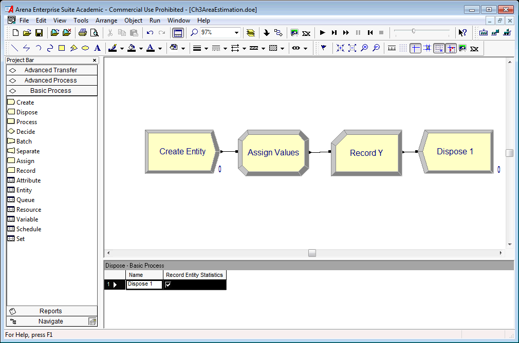
Figure 2.4: Arena model for estimating the area of f(x)= sqrt(x)
Figure 2.4 represent the flow chart solution within the environment. Notice the CREATE, ASSIGN, RECORD, and DISPOSE modules laid out in the model window. A CREATE module creates entities that flow through other modules. Figure 2.5 illustrates the creating of 1 entity by setting the maximum number of entities field to the value 1. Since the First Creation field has a value of 0.0, there will be 1 entity that is created at time 0. The CREATE module will be discussed in further detail, later in this chapter. The created entity will move to the next module (ASSIGN) and cause its logic to be executed.
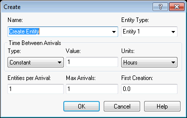
Figure 2.5: Creating 1 entity with a CREATE module
An ASSIGN module permits the assignment of values to various quantities of interest in the model. In Figure 2.6, a listing of the assignments for generating the value of \(x\), computing \(f(x)\), and \(y\) are provided. Each assignment is executed in the order listed. It is important to get the order correct when you write your programs!
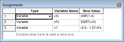
Figure 2.6: Making assignments using an ASSIGN module
Figure 2.7 shows the RECORD module for this situation. The value of the variable \(vY\) is in the Value text field. Because the Type of the record is set at Expression, the value of this variable will be observed every time an entity passes through the module. The observations will be tabulated so that the sample average and 95% half-width will be reported automatically on the output reports, labeled by the text in the Tally Name field. The results are illustrated in Figure 2.8.
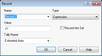
Figure 2.7: Recording statistics on an expression using a RECORD module
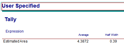
Figure 2.8: Results from the area estimation model
In order to run the model, you must indicate the required number of observations. Since each run of the model produces 1 entity and thus 1 observation, you need to specify the number of times that you want to run the model. This is accomplished using the Run Setup menu item. Figure 2.9 shows that the model is set to run for 20 replications. Replications will be discussed later in the text, but for now, you can think of a replication as a running of the model to produce observations. Each replication is independent of other replications. Thus, the observations across replications form a random sample of the observations. Arena will automatically report the statistics across the replications.
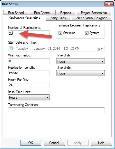
Figure 2.9: Setting up the simulation to replicate 20 observations
Figure 2.8 shows the results of estimating the area of the curve. Notice that the average value (4.3872) reported for the variable observed in the RECORD module is close to the true value of \(4.6\bar{6}\) computed for Example 2.1. The difference between the estimated value and the true value is due to sampling error. We will discuss how to control sampling error within Chapter 3. The area estimation model can be found within this Chapter’s files as AreaEstimation.doe.
Now let’s look at a slightly more complex static simulation.
2.2.4 The News Vendor Problem
The news vendor model is a classic inventory model that allows for the modeling of how much to order for a decision maker facing uncertain demand for an upcoming period of time. It takes on the news vendor moniker because of the context of selling newspapers at a newsstand. The vendor must anticipate how many papers to have on hand at the beginning of a day so as to not run short or have papers left over. This idea can be generalized to other more interesting situations (e.g. air plane seats). Discussion of the news vendor model is often presented in elementary textbooks on inventory theory. The reader is referred to (Muckstadt and Sapras 2010) for a discussion of this model.
The basic model is considered a single period model; however, it can be extended to consider an analysis covering multiple (or infinite) future periods of demand. The representation of the costs within the modeling offers a number of variations.
Let \(D\) be a random variable representing the demand for the period. Let \(F(d)= P[D \leq d]\) be the cumulative distribution function for the demand. Define \(G(q,D)\) as the profit at the end of the period when \(q\) units are ordered at the start of the period with \(D\) units of demand. The parameter \(q\) is the decision variable associated with this model. Depending on the value of \(q\) chosen by the news vendor, a profit or loss will occur.
There are two cases to consider \(D \geq q\) or \(D < q\). That is, when demand is greater than or equal to the amount ordered at the start of the period and when demand is less than the amount ordered at the start of the period. If \(D \geq q\) the news vendor runs out of items, and if \(D < q\) the news vendor will have items left over.
In order to develop a profit model for this situation, we need to define some model parameters. In addition, we need to determine the amount that we might be short and the amount we might have left over in order to determine the revenue or loss associated with a choice of \(q\). Let \(c\) be the purchase cost. This is the cost that the news vendor pays the supplier for the item. Let \(s\) be the selling price. This is the amount that the news vendor charges customers. Let \(u\) be the salvage value (i.e. the amount per unit that can be received for the item after the planning period). For example, the salvage value can be the amount that the news vendor gets when selling a left over paper to a recycling center. We assume that selling price \(>\) purchase cost \(>\) salvage value.
Consider the context of a news vendor planning for the day. What is the possible amount sold? If \(D\) is the demand for the day and we start with \(q\) items, then the most that can be sold is \(\min(D, q)\). That is, if \(D\) is bigger than \(q\), you can only sell \(q\). If \(D\) is smaller than \(q\), you can only sell \(D\).
What is the possible amount left over (available for salvage)? If \(D\) is the demand and we start with \(q\), then there are two cases: 1) demand is less than the amount ordered (\(D < q\)) or 2) demand is greater than or equal to the amount ordered (\(D \geq q\)). In case 1, we will have \(q-D\) items left over. In case 2, we will have \(0\) left over. Thus, the amount left over at the end of the day is \(\max(0, q-D)\). Since the news vendor buys \(q\) items for \(c\), the cost of the items for the day is \(c \times q\). Thus, the profit has the following form:
\[\begin{equation} G(D,q) = s \times \min(D, q) + u \times \max(0, q-D) - c \times q \tag{2.5} \end{equation}\]
In words, the profit is equal to the sales revenue plus the salvage revenue minus the ordering cost. The sales revenue is the selling price times the amount sold. The salvage revenue is the salvage value times the amount left over. The ordering cost is the cost of the items times the amount ordered. To find the optimal value of \(q\), we should try to maximize the expected profit. Since \(D\) is a random variable, \(G(D,q)\) is also a random variable. Taking the expected value of both sides of Equation (2.5), yields:
\[g(q) = E[G(D,q)] = sE[\min(D, q)] + uE[\max(0, q-D)] - cq\]
Whether or not this equation can be optimized depends on the form of the distribution of \(D\); however, simulation can be used to estimate this expected value for any given \(q\). Let’s look at an example.
Example 2.2 Sly’s convenience store sells BBQ wings for 25 cents a piece. They cost 15 cents a piece to make. The BBQ wings that are not sold on a given day are purchased by a local food pantry for 2 cents each. Assuming that Sly decides to make 30 wings a day, what is the expected revenue for the wings provided that the demand distribution is as show in Table 2.1.
| \(d_{i}\) | 5 | 10 | 40 | 45 | 50 | 55 | 60 |
|---|---|---|---|---|---|---|---|
| \(f(d_{i})\) | 0.1 | 0.2 | 0.3 | 0.2 | 0.1 | 0.05 | 0.05 |
| \(F(d_{i})\) | 0.1 | 0.3 | 0.6 | 0.8 | 0.9 | 0.95 | 1.0 |
The pseudo-code for the news vendor problem will require the generation of the demand from BBQ Wing demand distribution. In order to generate from this distribution, the DISC() function should be used. Since the cumulative distribution has already been computed, it is straight forward to write the inputs for the DISC() function. The function specification is:
\[\textit{DISC}(0.1,5,0.3,10,0.6,40,0.8,45,0.9,50,0.95,55,1.0,60)\]
Notice the pairs (\(F(d_{i})\), \(d_{i}\)). The final value of \(F(d_{i})\) must be the value 1.0.
First, let us define some variables to be used in the modeling: demand, amount sold, amount left at the end of the day, sales revenue, salvage revenue, price per unit, cost per unit, salvage per unit, and order quantity.
Let vDemand represent the daily demand
Let vAmtSold represent the amount sold
Let vAmtLeft represent the amount left at the end of the day
Let vSalesRevenue represent the sales revenue
Let vSalvageRevenue represent the salvage revenue
Let vPricePerUnit = 0.25 represent the price per unit
Let vCostPerUnit = 0.15 represent the cost per unit
Let vSalvagePerUnit = 0.02 represent the salvage value per unit
Let vOrderQty = 30 represent the amount ordered each day
The pseudo-code for this situation is as follows.
CREATE 1 entity
BEGIN ASSIGN
  vDemand = DISC(0.1,5,0.3,10,0.6,40,0.8,45,0.9,50,0.95,55,1.0,60)
  vAmtSold = MN(vDemand, vOrderQty)
  vAmtLeft = MX(0, vOrderQty - vDemand)
  vSalesRevenue = vAmtSold*vPricePerUnit
  vSalvageRevenue = vAmtLeft*vSalvagePerUnit
  vOrderingCost = vCostPerUnit*vOrderQty
  vProfit = vSalesRevenue + vSalvageRevenue - vOrderingCost
END ASSIGN
RECORD vProfit
DISPOSE
The CREATE module creates the an entity to represent the day. The ASSIGN modules implement the logic associated with the news vendor problem. The MN() function is used to compute the minimum of the demand and the amount ordered. The MX() function determines the amount unsold. The DISC() function implements the CDF of the demand in order to generate the daily demand. The rest of the equations follow directly from the previous discussion. The flow chart solution is illustrated in Figure 2.10 and uses the same flow chart modules (CREATE, ASSIGN, RECORD, DISPOSE) as in the last example.
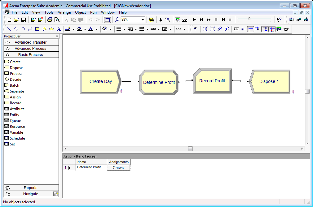
Figure 2.10: Model for news vendor problem
To implement the variable definitions from the pseudo-code, you need to use a VARIABLE module to provide the initial values of the variables. Notice in Figure 2.11 the definition of each variable and how the initial value of the variable vCostPerUnit is showing. The CREATE module is setup exactly as in the last example. The created entity will move to the next module (ASSIGN) illustrated in Figure 2.12. The assignments follow exactly the previously illustrate pseudo-code. Running the model for 100 days results in the output illustrated in Figure 2.13.
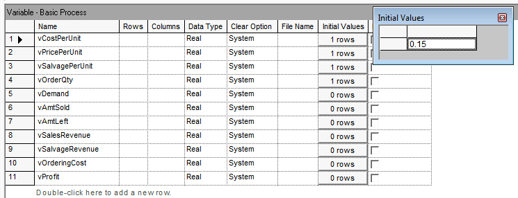
Figure 2.11: Variable definitions used in the news vendor solution
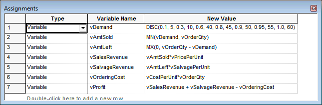
Figure 2.12: Assignments used in the news vendor solution
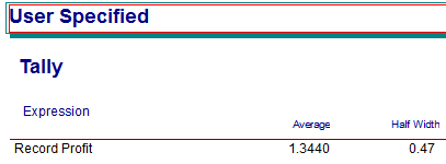
Figure 2.13: Results based on 100 replications of the news vendor model
The news vendor model can be found within this Chapter’s files as NewsVendor.doe.
In this section, we explored how to develop models in for which time is not a significant factor. In the case of the news vendor problem, where we simulated each day’s demand, time advanced at regular intervals. In the case of the area estimation problem, time was not a factor in the simulation. These types of simulations are often termed static simulation. In the next section, we begin our exploration of simulation where time is an integral component in driving the behavior of the system. In addition, we will see that time will not necessarily advance at regular intervals (e.g. hour 1, hour 2, etc.). This will be the focus of the rest of the book.