5.4 The Batch Means Method
In the batch mean method, only one simulation run is executed. After deleting the warm up period, the remainder of the run is divided into k batches, with each batch average representing a single observation as illustrated in Figure 5.24. In fact, this is essentially the same concept as previously discussed when processing the data using the Welch Plot Analyzer.
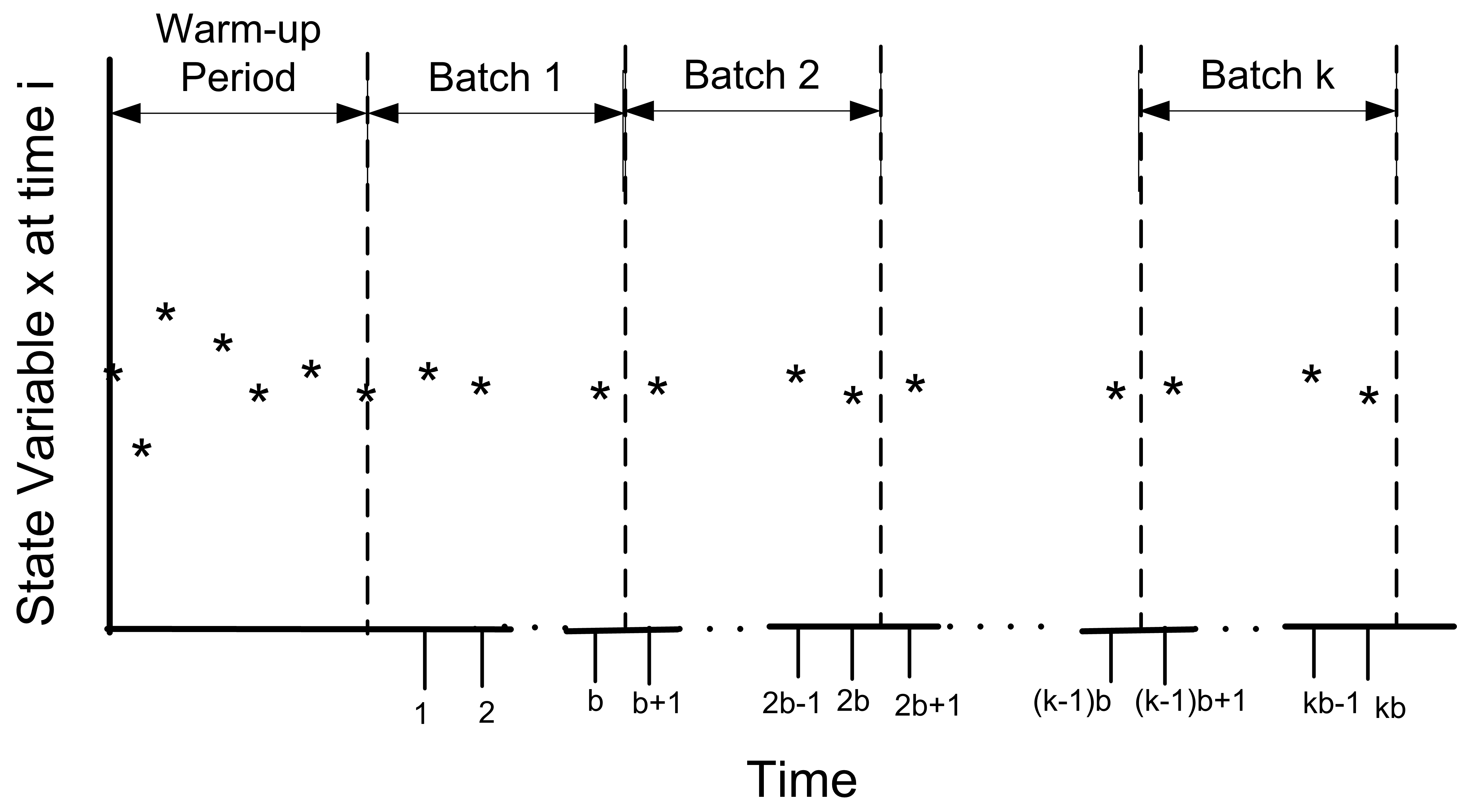
Figure 5.24: Illustration of the batch means concept
The advantages of the batch means method are that it entails a long simulation run, thus dampening the effect of the initial conditions. The disadvantage is that the within replication data are correlated and unless properly formed the batches may also exhibit a strong degree of correlation.
The following presentation assumes that a warm up analysis has already been performed and that the data that has been collected occurs after the warm up period. For simplicity, the presentation assumes observation based data. The discussion also applies to time-based data that has been cut into discrete equally spaced intervals of time as described in Section 5.3.1. Therefore, assume that a series of observations, \((X_1, X_2, X_3, \ldots, X_n)\), is available from within the one long replication after the warm up period. As shown earlier at the beginning of Section 5.1, the within replication data can be highly correlated. In that section, it was mentioned that standard confidence intervals based on the regular formula for the sample variance
\[S^2(n) = \dfrac{1}{n - 1}\sum_{i=1}^n (X_i - \bar{X})^2\]
are not appropriate for this type of data. Suppose you were to ignore the correlation, what would be the harm? In essence, a confidence interval implies a certain level of confidence in the decisions based on the confidence interval. When you use \(S^2(n)\) as defined above, you will not achieve the desired level of confidence because \(S^2(n)\) is a biased estimator for the variance of \(\bar{X}\) when the data are correlated. Under the assumption that the data are covariance stationary, an assessment of the harm in ignoring the correlation can be made. For a series that is covariance stationary, one can show that
\[Var(\bar{X}) = \dfrac{\gamma_0}{n}\left[1 + 2 \sum_{k=1}^{n-1} (1 - \dfrac{k}{n}) \rho_k\right]\]
where \(\gamma_0 = Var(X_i)\), \(\gamma_k = Cov(X_i, X_{i + k})\), and \(\rho_k = \gamma_k/\gamma_0\) for \(k = 1, 2, \ldots, n - 1\).
When the data are correlated, \(S^2/n\) is a biased estimator of \(Var(\bar{X})\). To show this, you need to compute the expected value of \(S^2/n\) as follows:
\[E\left[S^2/n\right] = \dfrac{\gamma_0}{n} \left[1 - \dfrac{2R}{n - 1}\right]\]
where
\[R = \sum_{k=1}^{n-1} (1 - \dfrac{k}{n}) \rho_k\]
Bias is defined as the difference between the expected value of the estimator and the quantity being estimated. In this case, the bias can be computed with some algebra as:
\[\text{Bias} = E\left[S^2/n\right] - Var(\bar{Y}) = \dfrac{-2 \gamma_0 R}{n - 1}\]
Since \(\gamma_0 > 0\) and \(n > 1\) the sign of the bias depends on the quantity R and thus on the correlation. There are three cases to consider: zero correlation, negative correlation, and positive correlation. Since \(-1 \leq \rho_k \leq 1\), examining the limiting values for the correlation will determine the range of the bias.
For positive correlation, \(0 \leq \rho_k \leq 1\), the bias will be negative, (\(- \gamma_0 \leq Bias \leq 0\)). Thus, the bias is negative if the correlation is positive, and the bias is positive if the correlation is negative. In the case of positive correlation, \(S^2/n\) underestimates the \(Var(\bar{X})\). Thus, using \(S^2/n\) to form confidence intervals will make the confidence intervals too short. You will have unjustified confidence in the point estimate in this case. The true confidence will not be the desired \(1 - \alpha\). Decisions based on positively correlated data will have a higher than planned risk of making an error based on the confidence interval.
One can easily show that for negative correlation, \(-1 \leq \rho_k \leq 0\), the bias will be positive (\(0 \leq Bias \leq \gamma_0\)). In the case of negatively correlated data, \(S^2/n\) over estimates the \(Var(\bar{X})\). A confidence interval based on \(S^2/n\) will be too wide and the true quality of the estimate will be better than indicated. The true confidence coefficient will not be the desired \(1 - \alpha\); it will be greater than \(1 - \alpha\).
Of the two cases, the positively correlated case is the more severe in terms of its effect on the decision making process; however, both are problems. Thus, the naive use of \(S^2/n\) for dependent data is highly unwarranted. If you want to build confidence intervals on \(\bar{X}\) you need to find an unbiased estimator of the \(Var(\bar{X})\).
The method of batch means provides a way to develop (at least approximately) an unbiased estimator for \(Var(\bar{X})\). Assuming that you have a series of data point, the method of batch means method divides the data into subsequences of contiguous batches:
\[\begin{gathered} \underbrace{X_1, X_2, \ldots, X_b}_{batch 1} \cdots \underbrace{X_{b+1}, X_{b+2}, \ldots, X_{2b}}_{batch 2} \cdots \\ \underbrace{X_{(j-1)b+1}, X_{(j-1)b+2}, \ldots, X_{jb}}_{batch j} \cdots \underbrace{X_{(k-1)b+1}, X_{(k-1)b+2}, \ldots, X_{kb}}_{batch k}\end{gathered}\]
and computes the sample average of the batches. Let \(k\) be the number of batches each consisting of \(b\) observations, so that \(k = \lfloor n/b \rfloor\). If \(b\) is not a divisor of \(n\) then the last \((n - kb)\) data points will not be used. Define \(\bar{X}_j(b)\) as the \(j^{th}\) batch mean for \(j = 1, 2, \ldots, k\), where,
\[\bar{X}_j(b) = \dfrac{1}{b} \sum_{i=1}^b X_{(j-1)b+i}\]
Each of the batch means are treated like observations in the batch means series. For example, if the batch means are re-labeled as \(Y_j = \bar{X}_j(b)\), the batching process simply produces another series of data, (\(Y_1, Y_2, Y_3, \ldots, Y_k\)) which may be more like a random sample. To form a \(1 - \alpha\)% confidence interval, you simply treat this new series like a random sample and compute approximate confidence intervals using the sample average and sample variance of the batch means series:
\[\bar{Y}(k) = \dfrac{1}{k} \sum_{j=1}^k Y_j\]
\[S_b^2 (k) = \dfrac{1}{k - 1} \sum_{j=1}^k (Y_j - \bar{Y})^2\]
\[\bar{Y}(k) \pm t_{\alpha/2, k-1} \dfrac{S_b (k)}{\sqrt{k}}\]
Since the original X’s are covariance stationary, it follows that the resulting batch means are also covariance stationary. One can show, see (Alexopoulos and Seila 1998), that the correlation in the batch means reduces as both the size of the batches, \(b\) and the number of data points, \(n\) increases. In addition, one can show that \(S_b^2 (k)/k\) approximates \(\text{Var}(\bar{X})\) with error that reduces as both \(b\) and \(n\) increase towards infinity.
The basic difficulty with the batch means method is determining the batch size or alternatively the number of batches. Larger batch sizes are good for independence but reduce the number of batches, resulting in higher variance for the estimator. (Schmeiser 1982) performed an analysis that suggests that there is little benefit if the number of batches is larger than 30 and recommended that the number of batches remain in the range from 10 to 30. However, when trying to access whether or not the batches are independent it is better to have a large number of batches (\(>\) 100) so that tests on the lag-k correlation have better statistical properties.
There are a variety of procedures that have been developed that will automatically batch the data as it is collected, see for example (Fishman and Yarberry 1997), (Steiger and Wilson 2002), and Banks et al. (2005). has its own batching algorithm. The batching algorithm is described in Kelton, Sadowski, and Sturrock (2004) page 311. See also (Fishman 2001) page 254 for an analysis of the effectiveness of the algorithm.
The discussion here is based on the description in Kelton, Sadowski, and Sturrock (2004). When the algorithm has recorded a sufficient amount of data, it begins by forming k = 20 batches. As more data is collected, additional batches are formed until k = 40 batches are collected. When 40 batches are formed, the algorithm collapses the number of batches back to 20, by averaging each pair of batches. This has the net effect of doubling the batch size. This process is repeated as more data is collected, thereby ensuring that the number of batches is between 20 and 39. The algorithm begins the formation of batches when it has at least 320 observations of tally-based data.
For time-persistent data, The algorithm requires that there were at least 5 time units during which the time-based variable changed 320 times. If there are not enough observations within a run then Insufficient is reported for the half-width value on the output reports. In addition, the algorithm also tests to see if the lag-1 correlation is significant by testing the hypothesis that the batch means are uncorrelated using the following test statistic, see (Alexopoulos and Seila 1998):
\[C = \sqrt{\dfrac{k^2 - 1}{k - 2}}\biggl[ \hat{\rho}_1 + \dfrac{[Y_1 - \bar{Y}]^2 + [Y_k - \bar{Y}]^2}{2 \sum_{j=1}^k (Y_j - \bar{Y})^2}\biggr]\]
\[\hat{\rho}_1 = \dfrac{\sum_{j=1}^{k-1} (Y_j - \bar{Y})(Y_{j+1} - \bar{Y})}{\sum _{j=1}^k (Y_j - \bar{Y})^2}\]
The hypothesis is rejected if \(C > z_\alpha\) for a given confidence level \(\alpha\). If the batch means do not pass the test, Correlated is reported for the half-width on the statistical reports.
5.4.1 Performing the Method of Batch Means
Performing the method of batch means in is relatively straight forward. The following assumes that a warm up period analysis has already been performed. Since batches are formed during the simulation run and the confidence intervals are based on the batches, the primary concern will be to determine the run length that will ensure a desired half-width on the confidence intervals. A fixed sampling based method and a sequential sampling method will be illustrated.
The analysis performed to determine the warm up period should give you some information concerning how long to make this single run and how long to set it’s warm up period. Assume that a warm up analysis has been performed using \(n_0\) replications of length \(T_e\) and that the analysis has indicated a warm up period of length \(T_w\).
As previously discussed, the method of replication deletion spreads the risk of choosing a bad initial condition across multiple replications. The method of batch means relies on only one replication. If you were satisfied with the warm up period analysis based on \(n_0\) replications and you were going to perform replication deletion, then you are willing to throw away the observations contained in at least \(n_0 \times T_w\) time units and you are willing to use the data collected over \(n_0 \times (T_e - T_w)\) time units. Therefore, the warm up period for the single replication can be set at \(n_0 \times T_w\) and the run length can be set at \(n_0 \times T_e\).
For example, suppose your warm up analysis was based on the initial results shown in Section 5.1, i.e. \(n_0\) = 10, \(T_e\) = 30000, \(T_w\) = 3000. Thus, your starting run length would be \(n_0 \times T_e = 10 \times 30,000 = 300,000\) and the warm period will be \(n_0 \times T_w = 30,000\). For these setting, the results shown in Figure 5.25 are very close to the results for the replication-deletion example.
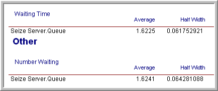
Figure 5.25: Initial batch means results.
Suppose now you want to ensure that the half-widths from a single
replication are less than a given error bound. The half-widths reported
by the simulation for a single replication are based on the batch
means. You can get an approximate idea of how much to increase the
length of the replication by using the functions: TNUMBAT(Tally ID) and
TBATSIZ(Tally ID) for observation based statistics or DNUMBAT(DSTAT ID)
and DBATSIZ(DSTAT ID) in conjunction with the half-width sample size
determination formula.
\[n \cong n_0 \left(\dfrac{h_0}{h}\right)^2\]
In this case, you interpret \(n\) and \(n_0\) as the number of batches. OUTPUT statistics can be added to the model to observe the number of batches for the waiting time in queue and for the size of each batch, as shown in Figure 5.26. The resulting values for the number of batches formed for the waiting times and the size of the batches are given in Figure 5.27 Using this information in the half-width based sample size formula with \(n_0 = 32\), \(h_0 = 0.06\), and \(h = 0.02\), yields:
\[n \cong n_0 \dfrac{h_0^2}{h^2} = 32 \times \dfrac{(0.06)^2}{(0.02)^2} = 288 \ \ \text{batches}\]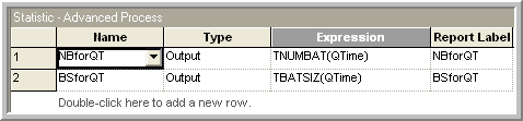
Figure 5.26: OUTPUT Statistics to get number of batches and batch size.
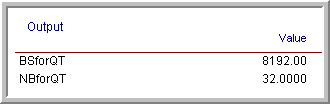
Figure 5.27: Results for number of batches and batch size.
Since each batch in the run had 8192 observations, this yields the need for additional observations for the waiting time in the queue. Since, in this model, customers arrive at a mean rate of 1 per minute, this requires about 2,359,296 additional time units of simulation. Because of the warm up period, you therefore need to set \(T_e\) equal to (2,359,296 + 30,000 = 2389296). Re-running the simulation yields the results shown in Figure 5.28. The results show that the half-width meets the desired criteria. This approach is approximate since you do not know how the observations will be batched when making the final run.
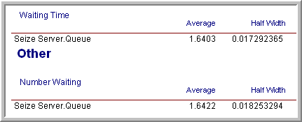
Figure 5.28: Batch means results for fixed sample size.
Rather than trying to fix the amount of sampling, you might instead try to use a sequential sampling technique that is based on the half-width computed during the simulation run. This is easy to do by supplying the appropriate expression within the Terminating Condition field on the Run Setup \(>\) Replication Parameters dialog.
Figure 5.29 illustrates that you can use a Boolean
expression within the Terminating Condition field. In this case, the
THALF(Tally ID) function is used to specify that the simulation should
terminate when the half-width criteria is met. The batching algorithm
computes the value of THALF(Tally ID) after sufficient data has been
observed. This expression can be expanded to include other performance
measures in a compound Boolean statement.
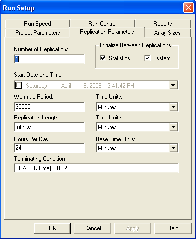
Figure 5.29: Sequential sampling using terminating condition.
The results of running the simulation based on the sequential method are given in Figure 5.30. In this case, the simulation run ended at approximately time 1,928,385. This is lower than the time specified for the fixed sampling procedure (but the difference is not excessive).
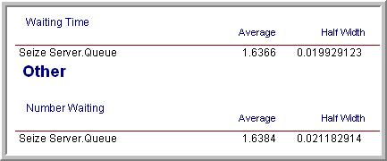
Figure 5.30: Results for infinite horizon sequential sampling method.
Once the warm up period has been analyzed, performing infinite horizon simulations using the batch means method is relatively straight forward. A disadvantage of this method is that it will be more difficult to use the statistical methods available within the Process Analyzer or within OptQuest because they assume a replication-deletion approach.
If you are faced with an infinite horizon simulation, then you can use either the replication-deletion approach or the batch means method. In either case, you should investigate if there may be any problems related to initialization bias. If you use the replication-deletion approach, you should play it safe when specifying the warm up period. Making the warm up period longer than you think it should be is better than replicating a poor choice. When performing an infinite horizon simulation based on one long run, you should make sure that your run length is long enough. A long run length can help to “wash out” the effects of initial condition bias.
Ideally, in the situation where you have to make many simulation experiments using different parameter settings of the same model, you should perform a warm up analysis for each design configuration. In practice, this is not readily feasible when there are a large number of experiments. In this situation, you should use your common sense to pick the design configurations (and performance measures) that you feel will most likely suffer from initialization bias. If you can determine long enough warm up periods for these configurations, the other configurations should be relatively safe from the problem by using the longest warm up period found.
There are a number of other techniques that have been developed for the analysis of infinite horizon simulations including the standardized time series method, the regenerative method, and spectral methods. An overview of these methods and others can be found in (Alexopoulos and Seila 1998) and in (Law 2007).
When performing an infinite horizon simulation analysis, we are most interested in the estimation of long-run (steady state) performance measures. In this situation, it can be useful to apply analytical techniques such as queueing theory to assist with determining whether or not the model is producing credible results. Even in the case of a finite horizon simulation, the steady state performance results from analytical models of queueing and inventory systems can be very helpful in understanding if the results produced by the simulation model make sense. In the next section, we apply the results of analytical queueing models from Appendix C to the simulation of a small manufacturing system in order to check the results of a simulation model. Being able to verify and validate a simulation model is a crucial skill to get your simulation models used in practice.