4.4 Statistical Issues When Comparing Two Systems
The previous sections have concentrated on estimating the performance of a system through the execution of a single simulation model. The running of the model requires the specification of the input variables (e.g. mean time between arrivals, service distribution, etc.) and the structure of the model (e.g. FIFO queue, process flow, etc.) The specification of a set of inputs (variables and/or structure) represents a particular system configuration, which is then simulated to estimate performance. To be able to simulate design configurations, you may have to build different models or you may be able to use the same model supplied with different values of the program inputs. In either situation, you now have different design configurations that can be compared. This allows the performance of the system to be estimated under a wide-variety of controlled conditions. It is this ability to easily perform these what-if simulations that make simulation such a useful analysis tool. Figure 4.59 represents the notion of using different inputs to get different outputs.
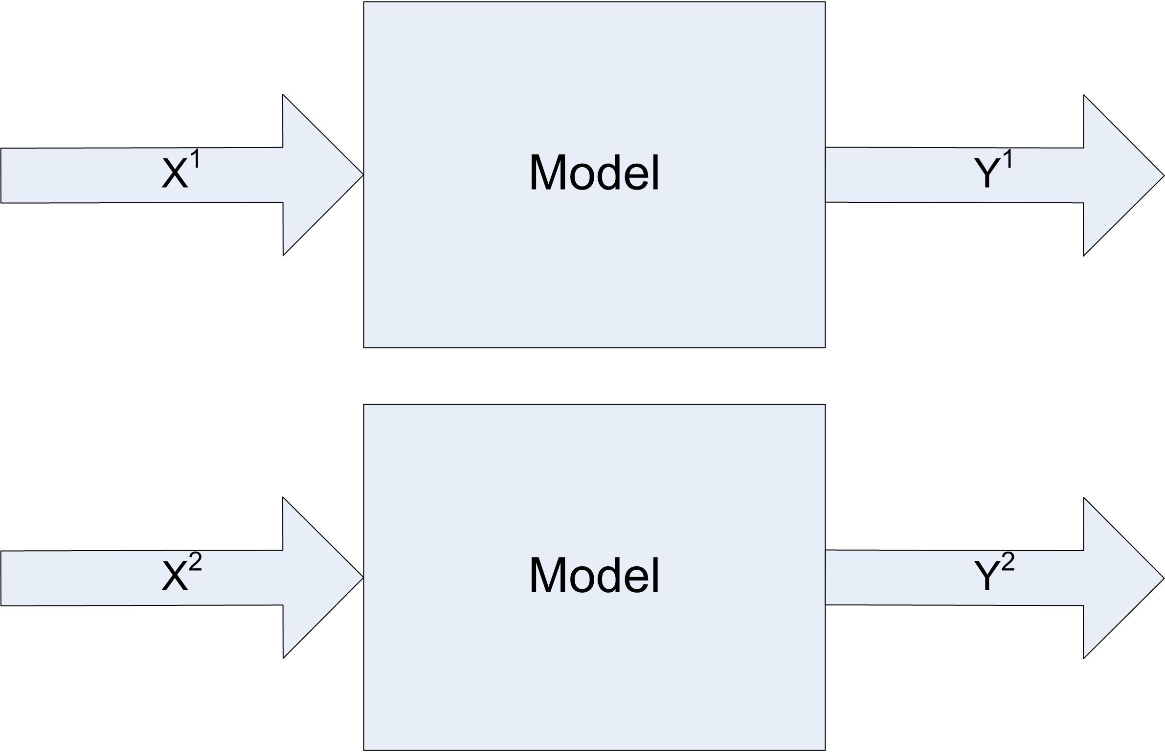
Figure 4.59: Changing inputs on models represent different system configurations
Naturally, when you have different design configurations, you would like to know which configurations are better than the others. Since the simulations are driven by random variables, the outputs from each configuration (e.g. \(Y^1, Y^2\)) are also random variables. The estimate of the performance of each system must be analyzed using statistical methods to ensure that the differences in performance are not simply due to sampling error. In other words, you want to be confident that one system is statistically better (or worse) than the other system.
The techniques for comparing two systems via simulation are essentially the same as that found in books that cover the statistical analysis of two samples (e.g. (Montgomery and Runger 2006)). This section begins with a review of these methods. Assume that samples from two different populations (system configurations) are available:
\[X_{11}, X_{12},\ldots, X_{1 n_1} \ \ \text{a sample of size $n_1$ from system configuration 1}\]
\[X_{21}, X_{22},\ldots, X_{2 n_2} \ \ \text{a sample of size $n_2$ from system configuration 2}\]
The samples represent a performance measure of the system that will be used in a decision regarding which system configuration is preferred. For example, the performance measure may be the average system throughput per day, and you want to pick the design configuration that has highest throughput.
Assume that each system configuration has an unknown population mean for the performance measure of interest, \(E[X_1] = \theta_1\) and \(E[X_2] = \theta_2\). Thus, the problem is to determine, with some statistical confidence, whether \(\theta_1 < \theta_2\) or alternatively \(\theta_1 > \theta_2\). Since the system configurations are different, an analysis of the situation of whether \(\theta_1 = \theta_2\) is of less relevance in this context.
Define \(\theta = \theta_1 - \theta_2\) as the mean difference in performance between the two systems. Clearly, if you can determine whether \(\theta >\) 0 or \(\theta <\) 0 you can determine whether \(\theta_1 < \theta_2\) or \(\theta_1 > \theta_2\). Thus, it is sufficient to concentrate on the difference in performance between the two systems.
Given samples from two different populations, there are a number of ways in which the analysis can proceed based on different assumptions concerning the samples. The first common assumption is that the observations within each sample for each configuration form a random sample. That is, the samples represent independent and identically distributed random variables. Within the context of simulation, this can be easily achieved for a given system configuration by performing replications. For example, this means that \(X_{11}, X_{12},\ldots, X_{1 n_1}\) are the observations from \(n_1\) replications of the first system configuration. A second common assumption is that both populations are normally distributed or that the central limit theorem can be used so that sample averages are at least approximately normal.
To proceed with further analysis, assumptions concerning the population variances must be made. Many statistics textbooks present results for the case of the population variance being known. In general, this is not the case within simulation contexts, so the assumption here will be that the variances associated with the two populations are unknown. Textbooks also present cases where it is assumed that the population variances are equal. Rather than making that assumption it is better to test a hypothesis regarding equality of population variances.
The last assumption concerns whether or not the two samples can be considered independent of each other. This last assumption is very important within the context of simulation. Unless you take specific actions to ensure that the samples will be independent, they will, in fact, be dependent because of how simulations use (re-use) the same random number streams. The possible dependence between the two samples is not necessarily a bad thing. In fact, under certain circumstance it can be a good thing.
The following sections first presents the methods for analyzing the case of unknown variance with independent samples. Then, we focus on the case of dependence between the samples. Finally, how to use to do the work of the analysis will be illustrated.
4.4.1 Analyzing Two Independent Samples
Although the variances are unknown, the unknown variances are either equal or not equal. In the situation where the variances are equal, the observations can be pooled when developing an estimate for the variance. In fact, rather than just assuming equal or not equal variances, you can (and should) use an F-test to test for the equality of variance. The F-test can be found in most elementary probability and statistics books (see (Montgomery and Runger 2006)).
The decision regarding whether \(\theta_1 < \theta_2\) can be addressed by forming confidence intervals on \(\theta = \theta_1 - \theta_2\). Let \(\bar{X}_1\), \(\bar{X}_2\), \(S_1^2\), and \(S_2^2\) be the sample averages and sample variances based on the two samples (k = 1,2):
\[\bar{X}_k = \dfrac{1}{n_k} \sum_{j=1}^{n_k} X_{kj}\]
\[S_k^2 = \dfrac{1}{n_k - 1} \sum_{j=1}^{n_k} (X_{kj} - \bar{X}_k)^2\]
An estimate of \(\theta = \theta_1 - \theta_2\) is desired. This can be achieved by estimating the difference with \(\hat{D} = \bar{X}_1 - \bar{X}_2\). To form confidence intervals on \(\hat{D} = \bar{X}_1 - \bar{X}_2\) an estimator for the variance of \(\hat{D} = \bar{X}_1 - \bar{X}_2\) is required. Because the samples are independent, the computation of the variance of the difference is:
\[Var(\hat{D}) = Var(\bar{X}_1 - \bar{X}_2) = \dfrac{\sigma_1^2}{n_1} + \dfrac{\sigma_2^2}{n_2}\]
where \(\sigma_1^2\) and \(\sigma_2^2\) are the unknown population variances. Under the assumption of equal variance, \(\sigma_1^2 = \sigma_2^2 =\sigma^2\), this can be written as:
\[Var(\hat{D}) = Var(\bar{X}_1 - \bar{X}_2) = \dfrac{\sigma_1^2}{n_1} + \dfrac{\sigma_2^2}{n_2} = \sigma^2 (\dfrac{1}{n_1} + \dfrac{1}{n_2})\]
where \(\sigma^2\) is the common unknown variance. A pooled estimator of \(\sigma^2\) can be defined as:
\[S_p^2 = \dfrac{(n_1 - 1)S_1^2 + (n_2 - 1)S_2^2}{n_1 + n_2 - 2}\]
Thus, a (\(1 - \alpha\))% confidence interval on \(\theta = \theta_1 - \theta_2\) is:
\[\hat{D} \pm t_{1-(\alpha/2) , v} s_p \sqrt{\dfrac{1}{n_1} + \dfrac{1}{n_2}}\]
where \(v = n_1 + n_2 - 2\). For the case of unequal variances, an approximate (\(1 - \alpha\))% confidence interval on \(\theta = \theta_1 - \theta_2\) is given by:
\[\hat{D} \pm t_{1-(\alpha/2) , v} \sqrt{S_1^2/n_1 + S_2^2/n_2}\]
where \[v = \Biggl\lfloor \frac{(S_1^2/n_1 + S_2^2/n_2)^2}{\frac{(S_1^2/n_1)^2}{n_1 +1} + \frac{(S_2^2/n_2)^2}{n_2 + 1}} - 2 \Biggr\rfloor\]
Let \([l, u]\) be the resulting confidence interval where \(l\) and \(u\) represent the lower and upper limits of the interval with by construction \(l < u\). Thus, if \(u < 0\), you can conclude with (\(1 - \alpha\))% confidence that \(\theta = \theta_1 - \theta_2 < 0\) (i.e. that \(\theta_1 < \theta_2\)). If \(l > 0\), you can conclude with (\(1 - \alpha\))% that \(\theta = \theta_1 - \theta_2 > 0\) (i.e. that \(\theta_1 > \theta_2\)). If \([l, u]\) contains 0, then no conclusion can be made at the given sample sizes about which system is better. This does not indicate that the system performance is the same for the two systems. You know that the systems are different. Thus, their performance will be different. This only indicates that you have not taken enough samples to detect the true difference. If sampling is relatively cheap, then you may want to take additional samples in order to discern an ordering between the systems.
Two configurations are under consideration for the design of an airport security checkpoint. A simulation model of each design was made. The replication values of the throughput per minute for the security station for each design are provided in Table 4.2.
| Design 1 | Design 2 | |
|---|---|---|
| 1 | 10.98 | 8.93 |
| 2 | 8.87 | 9.82 |
| 3 | 10.53 | 9.27 |
| 4 | 9.40 | 8.50 |
| 5 | 10.10 | 9.63 |
| 6 | 10.28 | 9.55 |
| 7 | 8.86 | 9.30 |
| 8 | 9.00 | 9.31 |
| 9 | 9.99 | 9.23 |
| 10 | 9.57 | 8.88 |
| 11 | 8.05 | |
| 12 | 8.74 | |
| \(\bar{x}\) | 9.76 | 9.10 |
| \(s\) | 0.74 | 0.50 |
| \(n\) | 10 | 12 |
Assume that the two simulations were run independently of each other, using different random numbers. Recommend the better design with 95% confidence.
According to the results:
\[\hat{D} = \bar{X}_1 - \bar{X}_2 = 9.76 - 9.1 = 0.66\]
In addition, we should test if the variances of the samples are equal. This requires an \(F\) test, with \(H_0: \sigma_{1}^{2} = \sigma_{2}^{2}\) versus \(H_1: \sigma_{1}^{2} \neq \sigma_{2}^{2}\). Based on elementary statistics, the test statistic is: \(F_0 = S_{1}^{2}/S_{1}^{2}\). The rejection criterion is to reject \(H_0\) if \(F_0 > f_{\alpha/2, n_1-1, n_2 -1}\) or \(F_0 < f_{1-(\alpha/2), n_1-1, n_2 -1}\), where \(f_{p, u, v}\) is the upper percentage point of the \(F\) distribution. Assuming a 0.01 significance level for the \(F\) test, we have \(F_0 = (0.74)^{2}/(0.50)^{2} = 2.12\). Since \(f_{0.005, 9, 11} = 5.54\) and \(f_{0.995, 9, 11} = 0.168\), there is not enough evidence to conclude that the variances are different at the 0.01 significance level. The value of \(f_{p, u, v}\) can be determined in as F.INV.RT(p, u, v) within Excel. Note also that \(f_{1-p, u, v} = 1/f_{p, v, u}\). In \(R\), the formula is \(f_{p, u, v} = qf(1-p, u,v)\), since \(R\) provides the quantile function, not the upper right tail function.
Since the variances can be assumed equal, we can use the pooled variance, which is:
\[\begin{aligned} S_p^2 & = \dfrac{(n_1 - 1)S_1^2 + (n_2 - 1)S_2^2}{n_1 + n_2 - 2}\\ & = \dfrac{(10 - 1)(0.74)^2 + (12 - 1)(0.5)^2}{12 + 10 - 2} \\ & = 0.384\end{aligned}\]
Thus, a (\(1 -0.05\))% confidence interval on \(\theta = \theta_1 - \theta_2\) is:
\[\begin{aligned} \hat{D} & \pm t_{1-(\alpha/2), v} s_p \sqrt{\dfrac{1}{n_1} + \dfrac{1}{n_2}} \\ 0.66 & \pm t_{1-0.025 , 20} (\sqrt{0.384}) \sqrt{\dfrac{1}{10} + \dfrac{1}{12}} \\ 0.66 & \pm (2.086)(0.6196)(0.428) \\ 0.66 & \pm 0.553\end{aligned}\]
where \(v = n_1 + n_2 - 2 = 10 + 12 - 2 = 20\). Since this results in an interval \([0.10, 1.21]\) that does not contain zero, we can conclude that design 1 has the higher throughput with 95% confidence.
The confidence interval can assist in making decisions regarding relative performance of the systems from a statistically significant standpoint. However, if you make a conclusion about the ordering of the system, it still may not be practically significant. That is, the difference in the system performance is statistically significant but the actual difference is of no practical use. For example, suppose you compare two systems in terms of throughput with resulting output \(\bar{X}_1\) = 5.2 and \(\bar{X}_2\) = 5.0 with the difference statistically significant. While the difference of 0.2 may be statistically significant, you might not be able to achieve this in the actual system. After all, you are making a decision based on a model of the system not on the real system. If the costs of the two systems are significantly different, you should prefer the cheaper of the two systems since there is no practical difference between the two systems. The fidelity of the difference is dependent on your modeling assumptions. Other modeling assumptions may overshadow such a small difference.
The notion of practical significance is model and performance measure dependent. One way to characterize the notion of practical significance is to conceptualize a zone of performance for which you are indifferent between the two systems. Figure 4.60 illustrates the concept of an indifference zone around the difference between the two systems. If the difference between the two systems falls in this zone, you are indifferent between the two systems (i.e. there is no practical difference).
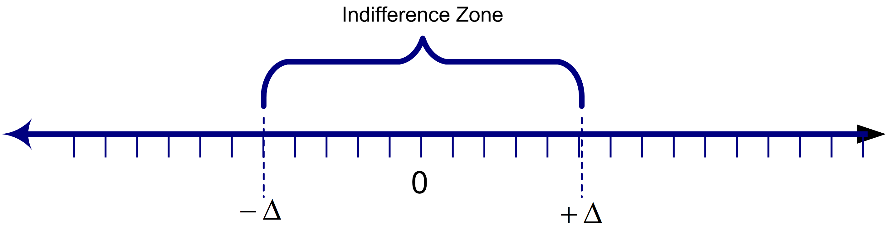
Figure 4.60: Concept of an indifference zone
Using the indifference zone to model the notion of practical significance, if \(u < -\Delta\), you can conclude confidence that \(\theta_1 < \theta_2\), and if \(l > \Delta\), you can conclude with confidence that \(\theta_1 > \theta_2\). If \(l\) falls within the indifference zone and \(u\) does not (or vice versa), then there is not enough evidence to make a confident conclusion. If \([l,u]\) is totally contained within the indifference zone, then you can conclude with confidence that there is no practical difference between the two systems.
4.4.2 Analyzing Two Dependent Samples
In this situation, continue to assume that the observations within a sample are independent and identically distributed random variables; however, the samples themselves are not independent. That is, assume that the \((X_{11}, X_{12},\), \(\ldots, X_{1n_1})\) and \((X_{21}, X_{22}, \ldots, X_{2n_2})\) from the two systems are dependent.
For simplicity, suppose that the difference in the configurations can be implemented using a simple parameter change within the model. For example, the mean processing time is different for the two configurations. First, run the model to produce \((X_{11}, X_{12}, \ldots, X_{1n_1})\) for configuration 1. Then, change the parameter and re-executed the model to produce \((X_{21}, X_{22}, \ldots, X_{2n_2})\) for configuration 2.
Assuming that you did nothing with respect to the random number streams, the second configuration used the same random numbers that the first configuration used. Thus, the generated responses will be correlated (dependent). In this situation, it is convenient to assume that each system is run for the same number of replications, i.e. \(n_1\) = \(n_2\) = n. Since each replication for the two systems uses the same random number streams, the correlation between \((X_{1,j}, X_{2,j})\) will not be zero; however, each pair will still be independent across the replications. The basic approach to analyzing this situation is to compute the difference for each pair:
\[D_j = X_{1j} - X_{2j} \ \ \text{for} \; j = 1,2,\ldots,n\]
The \((D_1, D_2, \ldots, D_n)\) will form a random sample, which can be analyzed via traditional methods. Thus, a (\(1 - \alpha\))% confidence interval on \(\theta = \theta_1 - \theta_2\) is:
\[\bar{D} = \dfrac{1}{n} \sum_{j=1}^n D_j\]
\[S_D^2 = \dfrac{1}{n-1} \sum_{j=1}^n (D_j - \bar{D})^2\]
\[\bar{D} \pm t_{1-\alpha/2, n-1} \dfrac{S_D}{\sqrt{n}}\]
The interpretation of the resulting confidence interval \([l, u]\) is the same as in the independent sample approach. This is the paired-t confidence interval presented in statistics textbooks.
Assume that the two simulations were run dependently using common random numbers. Recommend the better design with 95% confidence.
According to the results:
\[\bar{D} = \bar{X}_1 - \bar{X}_2 = 50.88 - 48.66 = 2.22\]
Also, we have that \(S_D^2 = (0.55)^2\). Thus, a (\(1 -0.05\))% confidence interval on \(\theta = \theta_1 - \theta_2\) is:
\[\begin{aligned} \hat{D} & \pm t_{1-(\alpha/2), n-1} \dfrac{S_D}{\sqrt{n}}\\ 2.22 & \pm t_{1-0.025 , 9} \dfrac{0.55}{\sqrt{10}}\\ 2.22 & \pm (2.261)(0.1739)\\ 2.22 & \pm 0.0.393\end{aligned}\]
Since this results in an interval \([1.827, 2.613]\) that does not contain zero, we can conclude that design 1 has the higher cost with 95% confidence.
Of the two approaches (independent versus dependent) samples, the latter is much more prevalent in simulation contexts. The approach is called the method of common random numbers (CRN) and is a natural by product of how most simulation languages handle their assignment of random number streams.
To understand why this method is the preferred method for comparing two systems, you need to understand the method’s affect on the variance of the estimator. In the case of independent samples, the estimator of performance was \(\hat{D} = \bar{X}_1 - \bar{X}_2\). Since
\[\begin{aligned} \bar{D} & = \dfrac{1}{n} \sum_{j=1}^n D_j \\ & = \dfrac{1}{n} \sum_{j=1}^n (X_{1j} - X_{2j}) \\ & = \dfrac{1}{n} \sum_{j=1}^n X_{1j} - \dfrac{1}{n} \sum_{j=1}^n X_{2j} \\ & = \bar{X}_1 - \bar{X}_2 \\ & = \hat{D}\end{aligned}\]
The two estimators are the same, when \(n_1 = n_2 = n\); however, their variances are not the same. Under the assumption of independence, computing the variance of the estimator yields:
\[V_{\text{IND}} = Var(\bar{X}_1 - \bar{X}_2) = \dfrac{\sigma_1^2}{n} + \dfrac{\sigma_2^2}{n}\]
Under the assumption that the samples are not independent, the variance of the estimator is:
\[V_{\text{CRN}} = Var(\bar{X}_1 - \bar{X}_2) = \dfrac{\sigma_1^2}{n} + \dfrac{\sigma_2^2}{n} - 2\text{cov}(\bar{X}_1, \bar{X}_2)\]
If you define \(\rho_{12} = corr(\bar{X}_1, \bar{X}_2)\), the variance for the common random number situation is:
\[V_{\text{CRN}} = V_{\text{IND}} - 2\sigma_1 \sigma_2 \rho_{12}\]
Therefore, whenever there is positive correlation \(\rho_{12} > 0\) within the pairs we have that, \(V_{\text{CRN}} < V_{\text{IND}}\).
If the variance of the estimator in the case of common random numbers is smaller than the variance of the estimator under independent sampling, then a variance reduction has been achieved. The method of common random numbers is called a variance reduction technique. If the variance reduction results in a confidence interval for \(\theta\) that is tighter than the independent case, the use of common random numbers should be preferred. The variance reduction needs to be big enough to overcome any loss in the number of degrees of freedom caused by the pairing. When the number of replications is relatively large (\(n > 30\)) this will generally be the case since the student-t value does not vary appreciatively for large degrees of freedom. Notice that the method of common random numbers might backfire and cause a variance increase if there is negative correlation between the pairs. An overview of the conditions under which common random numbers may work is given in (Law 2007).
This notion of pairing the outputs from each replication for the two system configurations makes common sense. When trying to discern a difference, you want the two systems to experience the same randomness so that you can more readily infer that any difference in performance is due to the inherent difference between the systems and not caused by the random numbers.
In experimental design settings, this is called blocking on a factor. For example, if you wanted to perform and experiment to determine whether a change in a work method was better than the old method, you should use the same worker to execute both methods. If instead, you had different workers execute the methods, you would not be sure if any difference was due to the workers or to the proposed change in the method. In this context, the worker is the factor that should be blocked. In the simulation context, the random numbers are being blocked when using common random numbers.
In the next section, we introduce a modeling situation involving the production of rings. We will then apply the methods of this section to compare two design configurations involving this system.