C.2 Examples and Applications of Queueing Analysis
The derivations and formulas in the previous section certainly appear to be intimidating and they can be tedious to apply. Fortunately, there is readily available software that can be used to do the calculations. On line resources for software for queueing analysis can be found at:
QTSPlus Excel based queueing theory software that accompanies Gross et al. (2008)
The most important part of performing a queueing analysis is to identify the most appropriate queueing model for a given situation. Then, software tools can be used to analyze the situation. This section provides a number of examples and discusses the differences between the systems so that you can better apply the results of the previous sections. The solutions to these types of problems involve the following steps:
Identify the arrival and service processes
Identify the size of the arriving population and the size of the system
Specify the appropriate queueing model and its input parameters
Identify the desired performance measures
Compute the required performance measures
C.2.1 Infinite Queue Examples
In this section, we will explore two queueing systems (M/M/1 and M/M/c) that have an infinite population of arrivals and an infinite size queue. The examples illustrate some of the common questions related to these types of queueing systems.
What is the probability that an arriving customer can enter one of the 3 spaces in front of the window?
What is the probability that an arriving customer will have to wait outside the 3 spaces?
What is the probability that an arriving customer has to wait?
How long is an arriving customer expected to wait before starting service?
How many car spaces should be provided in front of the window so that an arriving customer has a \(\gamma\) = 40% chance of being able to wait in one of the provided spaces?
Solution to Example C.1
The customers arrive according to a Poisson process, which implies that the time between arrivals is exponentially distributed. Thus, the arrival process is Markovian (M). The service process is stated as exponential. Thus, the service process is Markovian (M). There is only 1 window and customers wait in front of this window to receive service. Thus, the number of servers is \(c = 1\). The problem states that customers that arrive when the three spaces are filled, still wait for service outside the 3 spaces. Thus, there does not appear to be a restriction on the size of the waiting line. Therefore, this situation can be considered an infinite size system. The arrival rate is specified for any likely customer and there is no information given concerning the total population of the customers. Thus, it appears that an infinite population of customers can be assumed. We can conclude that this is a M/M/1 queueing situation with an arrival rate \(\lambda = 10/hr\) and a service rate of \(\mu = 12/hr\). Notice the input parameters have been converted to a common unit of measure (customers/hour).
The equations for the M/M/1 can be readily applied. From Section C.4 the following formulas can be applied:
\[ \begin{aligned} c & = 1\\ \lambda_n & = \lambda = 10/hr\\ \lambda_{e} & = \lambda \\ \mu_n & =\mu = 12/hr \\ \rho & = \dfrac{\lambda}{c\mu} = r = 10/12 = 5/6\\ P_0 & = 1 - \dfrac{\lambda}{\mu} = 1 - r = 1/6 \\ P_n & = P_0 r^n = \dfrac{1}{6} \left(\dfrac{5}{6}\right)^{n}\\ L & = \dfrac{r}{1 - r} = \dfrac{(5/6)}{1 - (5/6)} = 5\\ L_q & = \dfrac{r^2}{1 - r} = \dfrac{(5/6)^2}{1 - (5/6)} = 4.1\bar{6}\\ W_q & = \frac{L_q}{\lambda} = \frac{r}{\mu(1 - r)} = 0.41\bar{6} \; \text{hours} = 25.02 \; \text{minutes} \\ W & = \frac{L}{\lambda} = 5/10 = 0.5 \; \text{hours} = 30 \; \text{minutes} \\ \end{aligned} \]
Let’s consider each question from the problem in turn:
Probability statements of this form are related to the underlying state variable for the system. In this case, let \(N\) represent the number of customers in the system. To find the probability that an arriving customer can enter one of the 3 spaces in front of the window, you should consider the question: When can a customer enter one of the 3 spaces? A customer can enter one of the three spaces when there are 0 or 1 or 2 customers in the system. This is not \(N\) = 0, 1, 2, or 3 because if there are 3 customers in the system, then the \(3^{rd}\) space is taken. Therefore, \(P\lbrace N \leq 2 \rbrace\) needs to be computed.
To compute \(P[N \leq 2]\) note that:\[P[N \geq n] = \sum_{j=n}^{\infty} P_0 r^j = (1 - r)\sum_{j=n}^{\infty} r^{j-n} = (1 - r)\dfrac{r^n}{1 - r} = r^n\]
Therefore, \(P[N \leq n]\) is:
\[P[N \leq n] = 1 - P[N > n] = 1 - P[N \geq n + 1] = 1 - r^{n + 1}\]
Thus, we have that \(P[N \leq 2] = 1 - r^3 \cong 0.42\)
An arriving customer will have to wait outside of the 3 spaces, when there are more than 2 (3 or more) customers in the system. Thus, \(P[N > 2]\) needs to be computed to answer question (b). This is the complement event for part (a), \(P[N > 2] = 1 - P[N \leq 2] \cong 0.58\)
An arriving customer has to wait when there are 1 or more customers already at the pharmacy. This is \(P[N \geq 1]= 1 - P[N < 1] = 1 - P_0\).
\[P[N \geq 1] = 1 - P[N < 1] = 1 - P_0 = 1 - (1 - r) = \rho = \dfrac{5}{6}\]
The waiting time that does not include service is the queueing time. Thus, \(W_q\) needs to be computed to answer question (d).
\[W_q = 0.41\bar{6} \; \text{hours} = 25.02 \; \text{minutes}\]
This is a design question for which the probability of waiting in one of the provided spaces is used to determine the number of spaces to provide. Suppose that there are \(m\) spaces. An arriving customer can waiting in one of the spaces if there are \(m - 1\) or less customers in the system. Thus, \(m\) needs to be chosen such that \(P\lbrace N \leq m - 1\rbrace = 0.4\).
\[P[N \leq m - 1] = \gamma\] \[1 - r^m = \gamma\] \[r^m = 1 - \gamma\] \[m = \dfrac{\ln(1 - \gamma)}{\ln r} = \dfrac{\ln(1 - 0.4)}{\ln(\frac{5}{6})} = 2.8 \cong 3 \; \text{spaces}\]
Rounding up guarantees \(P[N \leq m - 1] \geq 0.4)\).
The following example models self-service copiers.
Solution to Example C.2
The Poisson arrivals and exponential service times make this situation an M/M/c where \(c\) is the number of copiers to install and \(\lambda = 0.5\) and \(\mu = 1/1.75\) per minute. To meet the design criteria, \(P[N \geq 4] = 1 - P[N \leq 3]\) needs to be computed for systems with \(c = 1,2,\ldots\) until \(P[N \geq 4]\) is less than 5%. This can be readily achieved with the provided formulas or by utilizing the aforementioned software. In what follows, the QTSPlus software was used.
The software is very self-explanatory. It is important to remember that when applying the queueing formulas make sure that you keep your time units consistent. Setting up the QTSPlus spreadsheet as shown in Figure C.6 with \(c=3\) yields the results shown in Figure C.7. By changing the number of servers, one can find that \(c=3\) meets the probability requirement as shown in Table C.2.
| \(c\) | \(P[N \geq 4] = 1 - P[N \leq 3]\) |
|---|---|
| 1 | 0.586182 |
| 2 | 0.050972 |
| 3 | 0.019034 |
| 4 | 0.013022 |
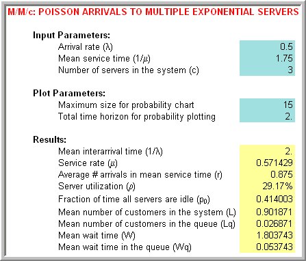
Figure C.6: QTSPlus M/M/c spreadsheet results
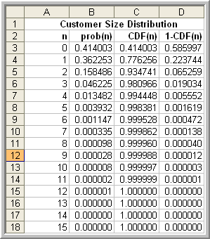
Figure C.7: QTSPlus M/M/c state probability results
C.2.1.1 Square Root Staffing Rule
Often in the case of systems with multiple servers such as the M/M/c, you want to determine the best value of \(c\), as in Example C.2. Another common design situation is to determine the value \(c\) of such that there is an acceptable probability that an arriving customer will have to wait. For the case of Poisson arrivals, this is the same as the steady state probability that there are more than c customers in the system. For the M/M/c model, this is called the Erlang delay probability:
\[P_w = P[N \geq c] = \sum_{n=c}^{\infty} P_n = \dfrac{\dfrac{r^c}{c!}}{\dfrac{r^c}{c!} + (1 - \rho)\sum_{j=0}^{c-1} \dfrac{r^j}{j!}}\]
Even though this is a relatively easy formula to use (especially in view of available spreadsheet software), an interesting and useful approximation has been developed called the square root staffing rule. The derivation of the square root staffing rule is given in (Tijms 2003). In what follows, the usefulness of the rule is discussed.
The square root staffing rule states that the least number of servers, \(c^{*}\), required to meet the criteria, \(P_w \leq \alpha\) is given by: \(c^{*} \cong r+ \gamma_\alpha\sqrt{r}\), where the factor \(\gamma_\alpha\) is the solution to the equation:
\[\dfrac{\gamma\Phi(\gamma)}{\varphi(\gamma)} = \dfrac{1 - \alpha}{\alpha}\]
The functions, \(\Phi(\cdot)\) and \(\varphi(\cdot)\) are the cumulative distribution function (CDF) and the probability density function (PDF) of a standard normal random variable. Therefore, given a design criteria, \(\alpha\), in the form a probability tolerance, you can find the number of servers that will result in the probability of waiting being less than \(\alpha\). This has very useful application in the area of call service centers and help support lines.
Solution to Example C.3
For \(\lambda = 0.5\) and \(\mu = 1/1.75\) per minute, you have that \(r = 0.875\). Figure C.8 illustrates the use of the SquareRootStaffingRule.xls spreadsheet that accompanies this chapter. The spreadsheet has text that explains the required inputs. Enter the offered load \(r\) in cell B3 and the delay criteria of 0.1 in cell B4. An initial search value is required in cell B5. The value of 1.0 will always work. The spreadsheet uses the goal seek functionality to solve for \(\gamma_\alpha\).
For this problem, this results in about 3 servers being needed to ensure that the probability of wait will be less than 10%. The square root staffing rule has been shown to be quite a robust approximation and can be useful in many design settings involving staffing.
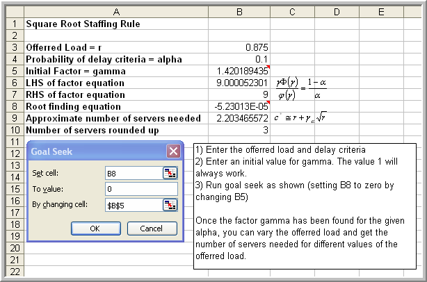
Figure C.8: Spreadsheet for square root staffing rule
The previous examples have had infinite system capacity. The next section presents examples of finite capacity queueing systems.
C.2.2 Finite Queue Examples
In this section, we will explore three queueing systems that are finite in some manner, either in space or in population. The examples illustrate some of the common questions related to these types of systems.
Solution to Example C.4
The finite buffer, Poisson arrivals, and exponential service times make this situation an M/M/1/6 where \(k = 6\) is the size of the system (5 in buffer + 1 in service) and \(\lambda =1\) and \(\mu = 1.2\) per minute. The desired performance measures are \(W\) and \(L\). Figure C.9 presents the results using QTSPlus. Notice that in this case, the effective arrival rate must be computed:
\[\lambda_e = \sum_{n=0}^{k-1} \lambda_n P_n = \sum_{n=0}^{k-1} \lambda P_n = \lambda\sum_{n=0}^{k-1} P_n = \lambda(1 - P_k)\]
Rearranging this formula, yields, \(\lambda = \lambda_e + \lambda_{f}\) where \(\lambda_{f} = \lambda P_k\) equals the mean number of customers that are turned away from the system because it is full. According to Figure C.9, the expected number of turned away because the system is full is about 0.077 per minute (or about 4.62 per hour).
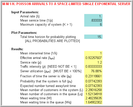
Figure C.9: Results for finite buffer M/M/1/6 queue
Let’s take a look at modeling a situation that we experience everyday, parking lots.
Solution to Example C.5
In this system, the parking spaces are the servers of the system. There are 10 parking spaces so that \(c = 10\). In addition, there is no waiting for one of the meters and thus no queue forms. Therefore, the system size, \(k\), is also 10. Because of the Poisson arrival process and exponential service times, this can be considered an M/M/10/10 queueing system. In other words, the size of the system is same as the number of servers, \(c = k = 10\).
In the case of a M/M/c/c queueing system, \(P_c\) represents the probability that all the servers in the system are busy. Thus, it also represents the probability that an arriving customer will be turned away. The formula for the probability of a lost customer is called the Erlang loss formula:
\[P_c = \frac{\frac{r^c}{c!}}{\sum_{n=0}^c \frac{r^n}{n!}}\]
Customers arrive at the rate \(\lambda = 20/hr\) whether the system is full or not. Thus, the expected number of lost customers per hour is \(\lambda P_c\). Since each customer brings \(1/\mu\) service time charged at \(w\) = $2 per hour, each arriving customer brings \(w/\mu\) of income on average; however, not all arriving customers can park. Thus, the university loses \(w \times 1/\mu \times \lambda P_c\) of income per hour. Figure C.10 illustrates the use of the QTSPlus software. In the figure the arrival rate of 40 per hour and the mean service time of 1 hours is entered. The number of parking spaces, 10, is the size of the system.
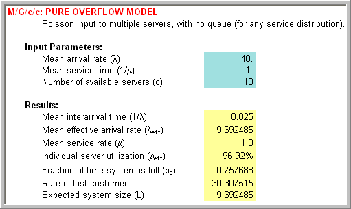
Figure C.10: Parking lot results for M/M/10/10 system
Thus according to Figure C.10, the university is losing about $2 \(\times\) 30.3 = $60.6 per hour because the metered lot is full during peak hours.
For this example, the service times are exponentially distributed. It turns out that for the case of \(c = k\), the results for the M/M/c/c model are the same for the M/G/c/c model. In other words, the form of the service time distribution does not matter. The mean of the service distribution is the critical input parameter to this analysis.
In the next example, a finite population of customers that can arrive, depart, and then return is considered. A classic and important example of this type of system is the machine interference or operator tending problem. A detailed discussion of the analysis and application of this model can be found in (Stecke 1992).
In this situation, a set of machines are tended by 1 or more operators. The operators must tend to stoppages (breakdowns) of the machines. As the machines breakdown, they may have to wait for the operator to complete the service of other machines. Thus, the machine stoppages cause the machines to interfere with the productivity of the set of machines because of their dependence on a common resource, the operator.
The situation that we will examine and for which analytical formulas can be derived is called the M/M/c/k/k queueing model where \(c\) is the number of servers (operators) and \(k\) is the number of machines (size of the population). Notice that the size of the system is the same as the size of the calling population in this particular model. For this system, the arrival rate of an individual machine, \(\lambda\), is specified. This is not the arrival rate of the population as has been previously utilized. The service rate of \(\mu\) for each operator is also necessary. The arrival and service rates for this system are:
\[\lambda_n = \begin{cases} (k - n) \lambda & n=0,1,2, \ldots k\\ 0 & n \geq k \end{cases}\]
\[\mu_n = \begin{cases} n \mu & n = 1,2,\ldots c\\ c \mu & n \geq c \end{cases}\]
These rates are illustrated in the state diagram of Figure C.11 for the case of 2 operators and 5 machines. Thus, for this system, the arrival rate to the system decreases as more machines breakdown. Notice that in the figure the arrival rate from state 0 to state 1 is \(5\lambda\). This is because there are 5 machines that are not broken down, each with individual rate, \(\lambda\). Thus, the total rate of arrivals to the system is \(5\lambda\). This rate goes down as more machines breakdown. When all the machines are broken down, the arrival rate to the system will be zero.
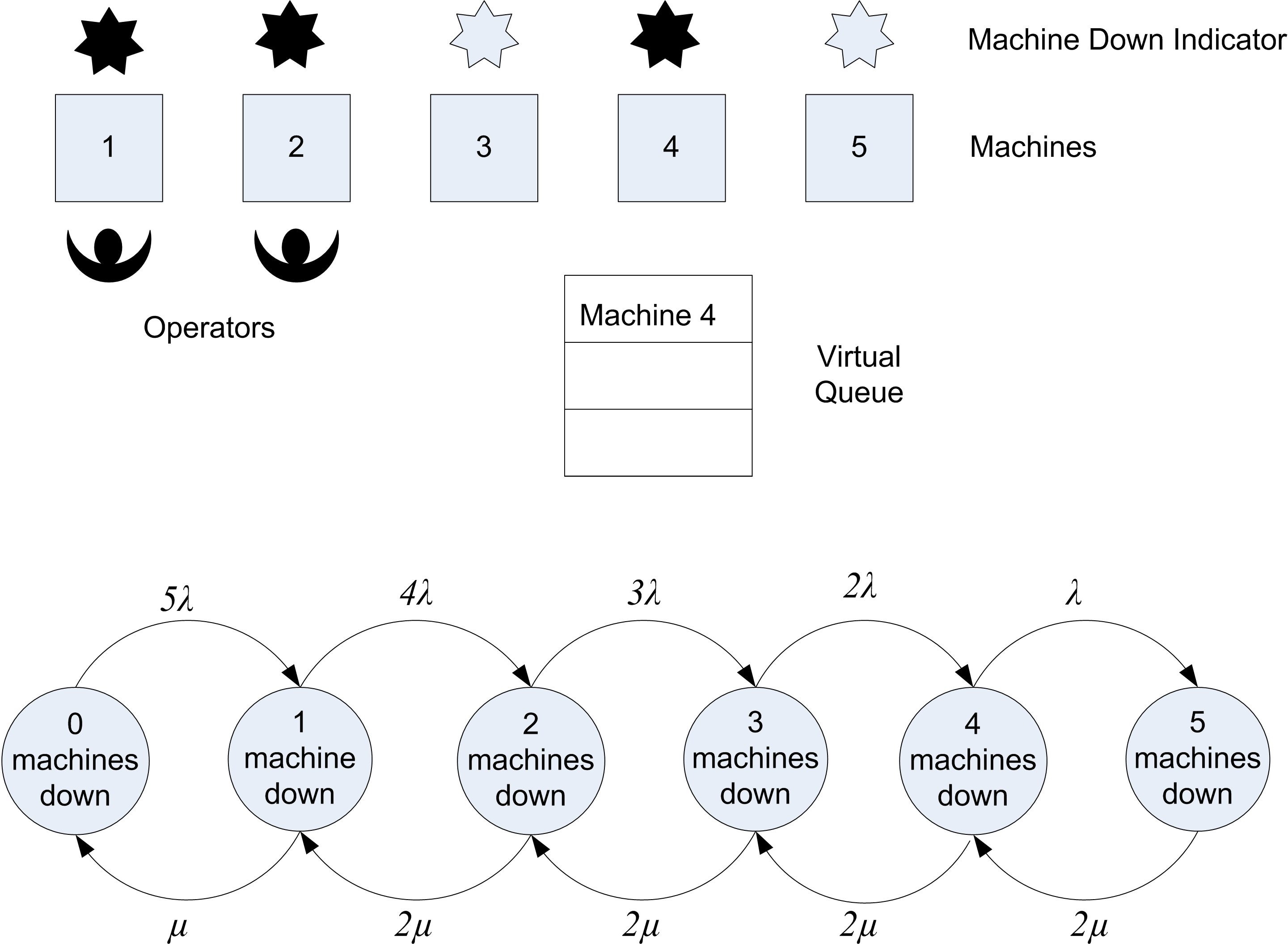
Figure C.11: System involving machine interference
Notice also that the service rate from state 1 to state 0 is \(\mu\). When one machine is in the system, the operator works at rate \(\mu\). Note also that the rate from state 2 to state 1 is \(2\mu\). This is because when there are 2 broken down machines the 2 operators are working each at rate \(\mu\). Thus, the rate of leaving from state 2 to 1 is \(2\mu\). Because there are only 2 operators in this illustration, the maximum rate is \(2\mu\) for state 2-5.
Notice that the customer in this system is the machine. Even though the machines do not actually move to line up in a queue, they form a virtual queue for the operators to receive their repair. Let’s consider an example of this system.
Solution to Example C.6
The arrival rate of an individual machine is \(\lambda = 1/10\) per hour and the service rate of \(\mu = 1/4\) per hour for each operator. In order to decide the most appropriate number of operators to tend the machines, a service criteria or a way to measure the cost of the system is required. Since costs are given, let’s formulate how much a given system configuration costs.
The easiest way to formulate a cost is to consider what a given system configuration costs on a per time basis, e.g. the cost per hour. Clearly, the system costs \(15 \times c\) ($/hour) to employ \(c\) operators. The problem also states that it costs $60/hour for each machine that is broken down. A machine is broken down if it is waiting for an operator or if it is being repaired by an operator. Therefore a machine is broken down if it is in the queueing system.
In terms of queueing performance measures, \(L\) machines can be expected to be broken down at any time in steady state. Thus, the expected steady state cost of the broken down machines is \(60 \times L\) per hour. The total expected cost per hour, \(E[\mathit{TC}]\), of operating a system configuration in steady state is thus:
\[E[\mathit{TC}] = 60 \times L + 15 \times c\]
Thus, the total expected cost, \(E[\mathit{TC}]\), can be evaluated for various values of \(c\) and the system that has the lowest cost determined.
Using the QTSPlus software, the necessary performance measures can be calculated and tabulated. Within the QTSPlus software you must choose the model category Multiple Servers and then choose the Markov Multi-Server Finite Source Queue without Spares model. Figure C.12 illustrates the inputs for the case of 1 server with 5 machines. Note that the software requests the time between arrivals, \(1/lambda\) and the mean service time, \(1/\mu\), rather than \(\lambda\) and \(\mu\).
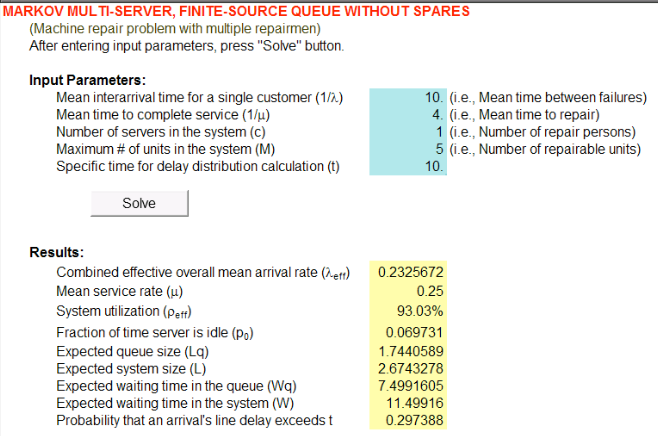
Figure C.12: Modeling the machine interference problem in QTSPlus
| \(\lambda\) | 0.10 | 0.10 | 0.10 | 0.10 | 0.10 |
| \(\mu\) | 0.25 | 0.25 | 0.25 | 0.25 | 0.25 |
| \(c\) | 1 | 2 | 3 | 4 | 5 |
| \(N\) | 5 | 5 | 5 | 5 | 5 |
| \(K\) | 5 | 5 | 5 | 5 | 5 |
| System | M/M/1/5/5 | M/M/2/5/5 | M/M/3/5/5 | M/M/4/5/5 | M/M/5/5/5 |
| \(L\) | 2.674 | 1.661 | 1.457 | 1.430 | 1.429 |
| \(L_q\) | 1.744 | 0.325 | 0.040 | 0.002 | 0.000 |
| \(B\) | 0.930 | 1.336 | 1.417 | 1.428 | 1.429 |
| \(B/c\) | 0.930 | 0.668 | 0.472 | 0.357 | 0.286 |
| \(E[\mathit{TC}]\) | $175.460 | $129.655 | $132.419 | $145.816 | $160.714 |
| \(\overline{\mathit{MU}}\) | 0.465 | 0.668 | 0.709 | 0.714 | 0.714 |
Table C.3 shows the results of the analysis. The results indicate that as the number of operators increase, the expected cost reaches its minimum at \(c = 2\). As the number of operators is increased, the machine utilization increases but levels off. The machine utilization is the expected number of machines that are not broken down divided by the number of machines:
\[\text{Machine Utilization} = \overline{\mathit{MU}} = \dfrac{k - L}{k} = 1 - \dfrac{L}{k}\]