6.3 Job Fair Example with Non-Stationary Arrivals
In Chapter 3, we modeled a STEM Career Fair Mixer and illustrated some of the basic modeling techniques associated with process modeling. For example, we saw how to generate entities (students) and have them experience simple processes before leaving the system. In Chapter 4, we embellished the STEM Mixer model by more realistically modeling the closing of the mixer and illustrated how to route entities within a system. In this section, we return to the STEM Career Fair Mixer model in order to illustrate the modeling of non-stationary arrivals and the collection of statistics for such situations. We will first update the system description to reflect the new situation and then discuss the building and analysis of the new model. In this new modeling situation, we will see how to utilize the SCHEDULE module for the case of varying the mean arrival rate and varying the resource capacity.
| Period | Time Frame | Duration | Mean Arrival Rate per Hour |
|---|---|---|---|
| 1 | 2 - 2:30 pm | 30 | 5 |
| 2 | 2:30 – 3 pm | 30 | 10 |
| 3 | 3 - 3:30 pm | 30 | 15 |
| 4 | 3:30 – 4 pm | 30 | 25 |
| 5 | 4 - 4:30 pm | 30 | 40 |
| 6 | 4:30 – 4 pm | 30 | 50 |
| 7 | 5 - 5:30 pm | 30 | 55 |
| 8 | 5:30 – 6 pm | 30 | 60 |
| 9 | 6 - 6:30 pm | 30 | 60 |
| 10 | 6:30 – 7 pm | 30 | 30 |
| 11 | 7 - 7:30 pm | 30 | 5 |
| 12 | 7:30 – 8 pm | 30 | 5 |
Because of the time varying nature of the arrival of students, the STEM mixer organizers have noticed that during the peak period of the arrivals there are substantially longer lines of students waiting to speak to a recruiter and often there are not enough tables within the conversation area for students. Thus, the mixer organizers would like to advise the recruiters as to how to staff their recruiting stations during the event. As part of the analysis, they want to ensure that 90 percent of the students experience an average system time of 35 minutes or less during the 4:30-6:30 pm time frame. They would also like to measure the average number of students waiting for recruiters during this time frame as well as the average number of busy recruiters at the MalWart and JHBunt recruiting stations. You should first perform an analysis based on the current staffing recommendations from the previous modeling and then compare those results to a staffing plan that allows the recruiters to change their assigned number of recruiters by hour. Everything else about the operation of the system remains the same as described in Chapter 4.
The solution to this modeling situation will put into practice the concepts introduced in the last two sections involving arrival schedules and resource schedules. That aspect of the modeling will turn out to be relatively straightforward. However, the requirement to collect statistics over the peak attendance period from 4:30 – 6:30 pm will require some new concepts on how to collect statistics by time periods.
6.3.1 Collecting Statistics by Time Periods
For some modeling situations, we need to be able to collect statistics during specific intervals of time. To be able to do this, we need to be able to observe what happens during those intervals. In general, to collect statistics during a particular interval of time will require the scheduling of events to observe the system (and its statistics) at the start of the period and then again at the end of the period in order to record what happened during the period. Let’s define some variables to clarify the concepts. We will start with a discussion of collecting statistics for tally-based data.
Let \(\left( x_{1},\ x_{2},x_{3},\cdots{,x}_{n(t)} \right)\) be a sequence of observations up to and including time \(t\).
Let \(n(t)\) be the number of observations up to and including time \(t\).
Let \(s\left( t \right)\) be the cumulative sum of the observations up to and including time \(t\). That is,
\[s\left( t \right) = \sum_{i = 1}^{n(t)}x_{i}\]
Let \(\overline{x}\left( t \right)\) be the cumulative average of the observations up to and including time \(t\). That is,
\[\overline{x}\left( t \right) = \frac{1}{n(t)}\sum_{i = 1}^{n(t)}x_{i} = \frac{s\left( t \right)}{n(t)}\]
We should note that we have \(s\left( t \right) = \overline{x}\left( t \right) \times n(t)\). Let \(t_{b}\) be the time at the beginning of a period (interval) of interest and let \(t_{e}\) be the time at the end of a period (interval) of interest such that \(t_{b} \leq t_{e}\). Define \(s(t_{b},t_{e}\rbrack\) as the sum of the observations during the interval, \((t_{b},t_{e}\rbrack\). Clearly, we have that,
\[s\left( t_{b},t_{e} \right\rbrack = s\left( t_{e} \right) - s\left( t_{b} \right)\]
Define \(n(t_{b},t_{e}\rbrack\) as the count of the observations during the interval, \((t_{b},t_{e}\rbrack\). Clearly, we have that,
\[n\left( t_{b},t_{e} \right\rbrack = n\left( t_{e} \right) - n\left( t_{b} \right)\]
Finally, we have that the average during the interval, \((t_{b},t_{e}\rbrack\) as
\[\overline{x}\left( t_{b},t_{e} \right\rbrack = \frac{s\left( t_{b},t_{e} \right\rbrack}{n\left( t_{b},t_{e} \right\rbrack}\]
Thus, if during the simulation we can observe, \(s\left( t_{b},t_{e} \right\rbrack\) and \(n\left( t_{b},t_{e} \right\rbrack\), we can compute the average during a specific time interval. To do this in a simulation, we can schedule an event for time, \(t_{b}\), and observe, \(s\left( t_{b} \right)\) and \(n\left( t_{b} \right)\). Then, we can schedule an event for time, \(t_{e}\), and observe, \(s\left( t_{e} \right)\) and \(n\left( t_{e} \right)\). Once these values are captured, we can compute \(\overline{x}\left( t_{b},t_{e} \right\rbrack\). If we observe this quantity across multiple replications, we will have the average that occurs during the defined period.
So far, the discussion has been about tally-based data. The process is essentially the same for time-persistent data. Recall that a time-persistent variable typically takes on the form of a step function. For example, let \(y(t)\) represents the value of some state variable at any time \(t\). Here \(y(t)\) will take on constant values during intervals of time corresponding to when the state variable changes, for example. \(y(t)\) = {0, 1, 2, 3, …}. \(y(t)\) is a curve (a step function in this particular case) and we compute the time average over the interval \((t_{b},t_{e}\rbrack\).as follows.
\[\overline{y}\left( t_{b},t_{e} \right) = \frac{\int_{t_{b}}^{t_{e}}{y\left( t \right)\text{dt}}}{t_{e} - t_{b}}\]
Similar to the tally-based case, we can define the following notation. Let \(a\left( t \right)\) be the cumulative area under the state variable curve.
\[a\left( t \right) = \int_{0}^{t}{y\left( t \right)\text{dt}}\]
Define \(\overline{y}(t)\) as the cumulative average up to and including time \(t\), such that:
\[\overline{y}\left( t \right) = \frac{\int_{0}^{t}{y\left( t \right)\text{dt}}}{t} = \frac{a\left( t \right)}{t}\]
Thus, \(a\left( t \right) = t \times \overline{y}\left( t \right)\). So, if we have a function to compute \(\overline{y}\left( t \right)\) we have the ability to compute,
\[\overline{y}\left( t_{b},t_{e} \right) = \frac{\int_{t_{b}}^{t_{e}}{y\left( t \right)\text{dt}}}{t_{e} - t_{b}} = \frac{a\left( t_{e} \right) - a\left( t_{b} \right)}{t_{e} - t_{b}}\]
Again, a strategy of scheduling events for \(t_{b}\) and \(t_{e}\) can allow you to observe the required quantities at the beginning and end of the period and then observe the desired average.
The key to collecting the statistics on observation-based over an
interval of time within Arena is the usage of the TAVG(tally ID) and the TNUM(tally ID) functions within Arena. The tally ID is the name of the corresponding
tally variable, typically defined within the RECORD module or when
defining a Tally set. Using the previously defined notation, we can note
the following: TAVG(tally ID) = \(\overline{x}\left( t \right)\) and
TNUM(tally ID) = \(n(t)\). Thus, we can compute s(t) for some tally
variable via:
\(s(t)\)=TAVG(tally ID)*TNUM(tally ID)
Given that we have the ability to observe \(n(t)\) and \(s(t)\) via these functions, we have the ability to collect the period statistics for any interval.
To make this more concrete, let’s collect statistics for every hour of
the day for an 8-hour simulation. In what follows, we will outline via
pseudo-code how to implement this situation. Suppose we are interested
in collecting the average time customers spend in a queue for a simple
single server queueing system (e.g. a M/M/1 queue) for each hour of an 8
hour day. Let’s call the queue, ServerQ and define a tally variable
called QTimeTally that collects the average time in the queue.
The first step is to define a clock entity that can keep track of each
hour of the day. We will use the clock entity to schedule the events and
record the desired statistics for each period. The clock entity will
loop after delaying for the period length and increment the period
indicator. At the end of the period, we will tabulate \(n(t)\) and \(s(t)\)
using TAVG() and TNUM(), compute the average during the period and then
prepare for the next hour by saving the cumulative statistics.
First, we define the variables, attributes and sets that we are going to use.
VARIABLES:
// to keep track of the current hour, the 0th hour is the 1st period
vPeriod

Attributes:
mySum// the cumulative sum at the beginning of the period
myNum // the cumulative number at the beginning of the period
myPeriodSum // the sum during the period
myPeriodNum // the count during the period
myPeriodAvg // the average computed within the period

Sets:
WaitTimeTallySet as a tally set with 8 elements, 1 for each period
(hour) of the day
Then, the pseudo-code for the clock-entity operation is as follows:
CREATE 1 entity at time 0.0
A: ASSIGN vPeriod = vPeriod + 1
mySum = 0.0
myNum = 0
DELAY for 1 hour
BEGIN ASSIGN
// collect the cumulative sum and count
myPeriodSum = TAVG(QTimeTally)*TNUM(QTimeTally) - mySum
myPeriodNum = TNUM(QTimeTally) - myNum
// save the current sum again for next period
mySum = TAVG(QTimeTally)*TNUM(QTimeTally)
myNum = TNUM(QTimeTally)
END ASSIGN
DECIDE IF myPeriodNum > 0
 RECORD (myPeriodSum/myPeriodNum) by Set: WaitTimeTallySet using index, vPeriod
END DECIDE
Go To: A
If there are multiple performance measures that need collecting, then this kind of logic can be repeated. In addition, by using sets, arrays, or arrayed expressions, you could define many variables and loop through all that are necessary to compute many performance measures for the periods. This can become quite tedious for a large number of performance measures. Also, note that the above logic assumes that we are simulating the system of interest for 8 hours, such that the replication length is set at 8 hours and the simulation will stop at that time. If you are collecting statistics for periods of time that do not span the entire simulation run length, then you need to provide additional logic for the clock-entity so that you ensure valid collection intervals.
Finally, to compute the time-persistent averages within Arena we can
proceed in a very similar fashion as previously described by using the
DAVG(Dstat ID) function. The DAVG(Dstat ID) function is
\(\overline{y}\left( t \right)\) the cumulative average of a
time-persistent variable. Thus, we can easily compute
\(a\left( t \right) = t \times \overline{y}\left( t \right)\) via
DAVG(Dstat ID)*TNOW. Therefore, we can use the same strategy as noted
in the illustrative pseudo-code to compute the time average over a given
period of time, \(\overline{y}\left( t_{b},t_{e} \right).\)
Fortunately, Arena has a method to automate this approach within the
STATISTIC module on the Advanced Process Panel. Within the module you
can define a time-persistent statistic and then provide a pattern for
collecting the average over user defined periods. The Smarts file,
“Statistics Capturing Variable Metric over a specified Time Period.doe”
illustrates the use of this option. In the dialog shown here, the
variable, vMoney_in_the_Bank, is observed starting at time 3 hours after
the simulation starts, with an observation period of 3 hours. In
addition, the observation is repeated every 8 hours. That is, after an
8-hour period, we start the observation period of 3 hours again. For
additional details, the interested reader should refer to the Arena Help
on these options, which will provide more of the technical details of
the meaning of the various options. We will illustrate the use of this
functionality when developing the updated STEM Mixer model.
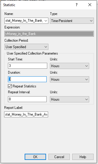
Figure 6.16: Capturing variable metric over a specified time period
6.3.2 Modeling the Statistical Collection
Now that we have a better understanding of the statistical collection requirements for the revised STEM mixer situation, we can build the model. First, we will outline the collection of the statistics during the peak period using the concepts from the last section. Then, we will implement the model using Arena.
The pseudo-code for this situation is actually simpler than illustrated in the last section because we only have to collect statistics during the peak period and it occurs only once during the 6 hour operating horizon. In what follows, we will collect both the system time and the average number of students waiting for a recruiter during the peak period. We will also see how to collect the average number waiting during the peak period using Arena’s STATISTIC module.
Define the following additional variables, attributes, and statistics to add to the existing STEM Mixer model of Chapter 4.
VARIABLES:
// time that the period starts, e. g. 4:30
vTimeOfPeriodStart = 150 minutes
// the length of the peak period
vPeakPeriodLength = 120 minutes

ATTRIBUTES:
// cumulative sum for system time at the beginning of the peak period
myCumSumSysTime
// cumulative number of system time observations at the beginning of the peak period
myCumNumSysTime
// cumulative area of the number of students waiting at the beginning of the peak period
myCumAreaWaitingStudents

TALLIES:
Tally System Time

TIME PERSISTENT Statistics:
NumStudentsWaitingTP, NQ(MalMart) + NQ(JHBunt)
Now, we can outline the modeling to collect the statistics by period.
CREATE 1 entity at time vTimeOfPeriodStart
BEGIN ASSIGN
  myCumSumSysTime = TAVG(Tally System Time)*TNUM(Tally System Time)
  myCumNumSysTime = TNUM(Tally System Time)
  myCumAreaWaitingStudents = DSTAT(NumStudentsWaitingTP)*TNOW
END ASSIGN
DELAY vPeakPeriodLength minutes
BEGIN ASSIGN
  myPeriodSum = TAVG(Tally System Time)*TNUM(Tally System Time) - myCumSumSysTime
  myPeriodNum = TNUM(Tally System Time) - myCumNumSysTime
  myPeriodArea = DSTAT(NumStudentsWaitingTP)*TNOW - myCumAreaWaitingStudents
END ASSIGN
DECIDE IF myPeriodNum > 0
 RECORD (myPeriodSum/myPeriodNum) as SystemTimeDuringPeriod
END DECIDE
RECORD (myPeriodArea/vPeakPeriodLength) as TimeAvgNumWaitingDuringPeriod
DISPOSE
Notice that within this pseudo-code, we only have the two events (one at the beginning and one at the end) of the delay representing the observation period in which to capture the statistics. Before the period delay, we capture the statistics at the beginning of the period. Then, after the period, we can compute what happened during the period and then record the statistics for the period. Also notice the use of variables to represent the peak period length and when the period starts. This allows these variables to be changed more easily if you decide to experiment with the parameter settings.
6.3.3 Implementing the Model in Arena
Now we are ready to implement the changes to the model developed in Chapter 4 section 4.1. There are really just two major changes to make 1) implementing the non-stationary arrivals and 2) implementing the statistical collection for the peak period. To start, we need to take the mean arrival rate information found in Example 6.1 and define a schedule for the arrival of students to the mixer.
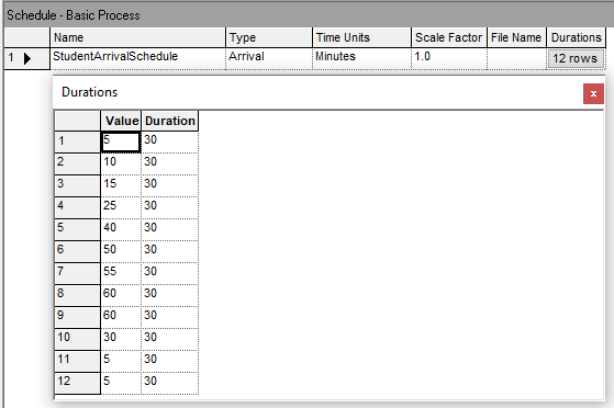
Figure 6.17: Student arrival schedule for 30 minute intervals
Figure 6.17 shows the Arena arrival schedule data sheet view. Because the time units are set to minutes, the (value, duration) pairs are entered with the duration values as 30 minutes. Also, because the arrival rate data is already per hour, we can simply enter the mean arrival rates. If the provide mean arrival rate data was not per hour, then we would have needed to convert them to a per hour basis before entering them into the arrival schedule. Next, the arrival schedule must be connected to the CREATE module used to create the student entities.
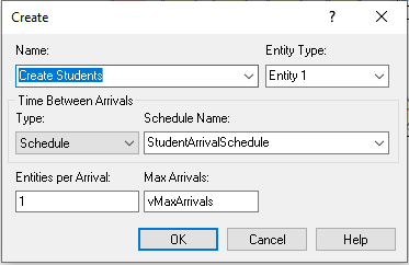
Figure 6.18: Updated CREATE module with arrival schedule
Figure 6.18 illustrates the updated CREATE module. Notice that the type of arrival has been designated as Schedule and the name of the schedule from Figure 6.17 has been supplied. As discussed in Chapter 4, we still turn off the CREATE module by setting vMaxArrivals to 0 by using an entity scheduled to occur at the end of the mixer. However, because we used an arrivals schedule we could also have specified one extra interval in the arrival schedule with the (rate, duration) pair as (0, ). A blank duration is interpreted as infinity. Thus, rate would be set the mean arrival rate to 0 when that interval occurs and it would remain at 0 for the remainder of the simulation. This would effectively shut off the CREATE module.
Now we will implement the pseudo-code of the last section within Arena. An overview of the Arena flow chart modules can be found in Figure 6.19.
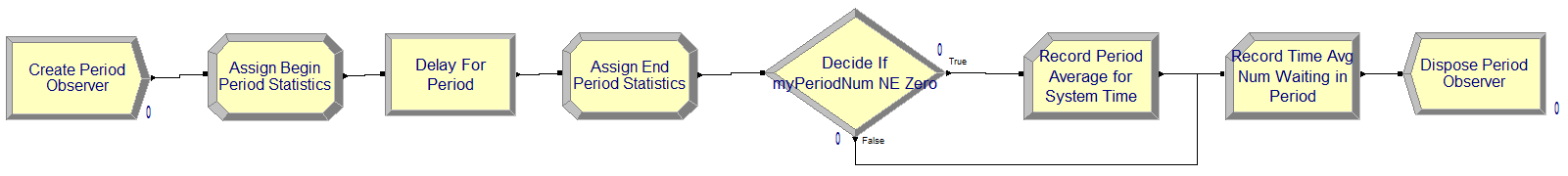
Figure 6.19: Overview of statistical collection logic
To implement this logic, we will first update the variables, attributes, and time persistent variables. Figure 6.20 and 6.21 show the updated attributes and variables to be used in the revised model. The variables and attribute names match what was presented in the pseudo-code.
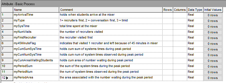
Figure 6.20: Updated attributes
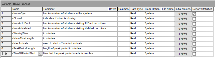
Figure 6.21: Updated variables
Figure 6.22 illustrates the updated definition of additional time persistent variables to collect statistics during various time periods. The two definitions on rows 2 and 3 collect the same performance measure, the average number of students waiting for either recruiter during the peak period. The definition on row 2 is used within the implementation of the previously discussed pseudo-code. The definition on row 3 will use Arena’s enhance statistical collect by period functionality to start the collection at time 150 and last for 120 minutes. We will see that the results of both methods for collecting this performance measure will match exactly.
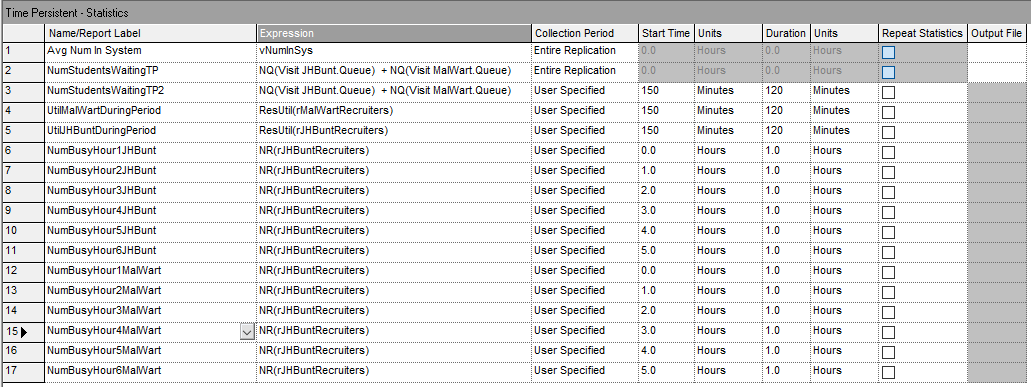
Figure 6.22: Updated time persistent statistic definitions
Then, there are additional time-persistent performance measures defined for the peak period and for the collection of hourly statistics. Rows 4 and 5 of Figure 6.22 collect the utilization of the resources used to model the JHBunt and MalMart recruiters using the ResUtil() function. This will allow us to note the utilization during the peak period. Then, rows 6 through 17 simply collect the average number of busy units of resource for JHBunt and MalMart for each hour of operation of the mixer. These statistics will facilitate determining how many recruiters to staff during each hour of operation.
To implement the modules found in Figure 6.19, we need to use CREATE, ASSIGN, DELAY, DECIDE, and RECORD modules that follow the previously described pseudo-code. Figure 6.23 shows the creating of the logical entity to collect statistics for the peak period.
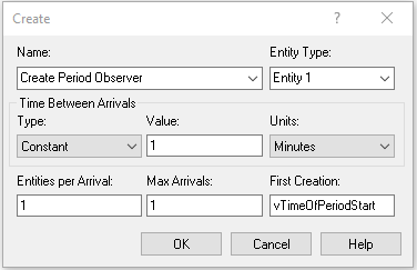
Figure 6.23: Creating the period observer
Figure 6.24 shows the ASSIGN modules used to capture the statistics at the beginning and end of the period. Notice the use of the TAVG(), TNUM(), and DAVG() functions as discussed in the pseudo-code.
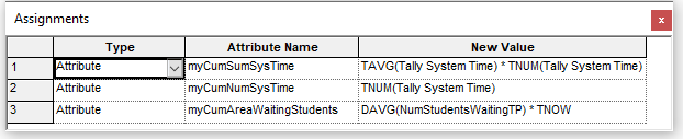
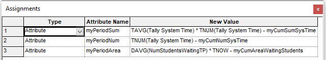
Figure 6.24: Assign logic to capture period Statistics
Figure 6.25 illustrates the use of a DECIDE module to check if there were no observations during the peak period in order to avoid a divide by zero error when computing the system time for the peak period.
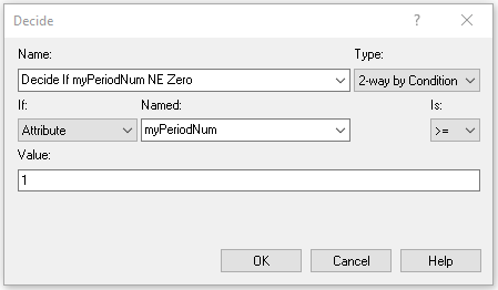
Figure 6.25: Checking for zero in the denominator
Figures 6.26 and 6.27 present the RECORD modules for capturing the peak period system time and average number of students waiting for either recruiter.
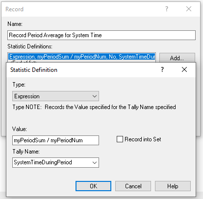
Figure 6.26: Updated time persistent statistic definitions
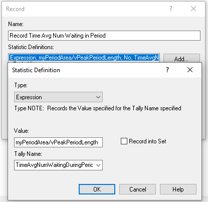
Figure 6.27: Updated time persistent statistic definitions
The entire Arena model is found in the file STEM_MixerArrivalsScheduleOnly.doe. This implementation has not yet considered the resource schedule constructs that were previously discussed. We will run this model and review the statistics to understand how to set up the resource capacity change. The base case scenario that we will perform is to run the model using the previously specified capacity of 3 units for JHBunt and 2 units for MalMart. We will see how the non-stationary arrivals affect the performance of the system.
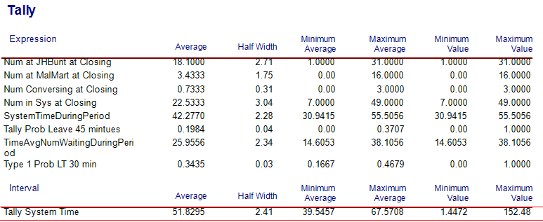
Figure 6.28: Base scenario tally results for non-stationary arrivals and no resource capacity change
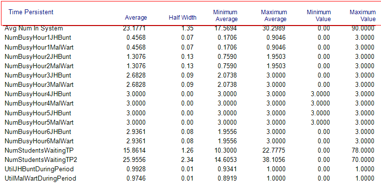
Figure 6.29: Base scenario time persistent results for non-stationary arrivals and no resource capacity change
Examining Figure 6.28, the first thing to note is that the overall system time for the students has increased to about 52 minutes versus the 27.6 minutes in Chapter 4. Clearly, the non-stationary arrival behavior of the students has a significant affect on the system and should be accounted for within the modeling. By looking at Figure 6.29, the reason for the increase in system time becomes clear. The utilization of the recruiting stations is nearly 100 percent (99% and 97%) during the peak period. Utilization this high will cause a significant line that will take some time to be worked down as the arrival rate eventually decreases. This can be better noted by reviewing the average number of busy units by hour of operation within Figure 6.29. Clearly, hours 4, 5, and 6 all have the reported average number busy very near or at the capacity limit of the resources. This indicates that we should increase the capacity during those time periods. Finally, please note the value of the statistic, TimeAvgNumWaitingDuringPeriod on Figure 6.28 of 25.9556. In addition, note on Figure 6.29, the value of time-persistent statistic, NumStudentsWaitingTP2, as also 25.9556. We see that the two methods of capturing this statistic via the by hand method and by enhanced functionality for period based collection of time-persistent statistics resulted in exactly the same estimates. Now you can better understand what Arena is doing to collect period based statistics.
A easy way to further analyze this situation is to set the capacity of the resources to infinity and review the estimated number of busy resources by hour of the day. Then, we can specify a capacity by hour that results in a desired utilization for each hour of the day.
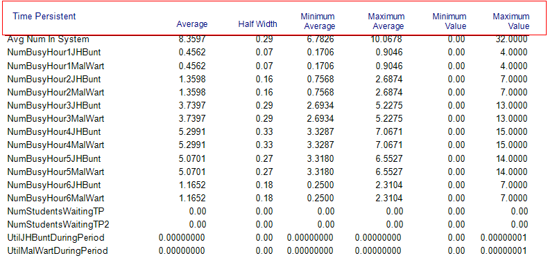
Figure 6.30: Base scenario time persistent results for non-stationary arrivals and infinite resource capacity
Figure 6.30 shows the result of running the non-stationary arrival schedule with infinite capacity for the recruiting resources. Notice how the estimated number busy units for the resources track the arrival pattern. Now considering the JHBunt recruiting station during the fourth hour of the day, we see an average number of recruiters busy of 5.2991. Thus, if we set the resource capacity of the JHBunt recruiting station to 6 recruiters during the fourth hour of the day, we would expect to achieve a utilization of about 88%, (\(5.2991/6 = 0.8832\)). With this thinking in mind we can determine the capacity for each hour of the day and the expected utilization.
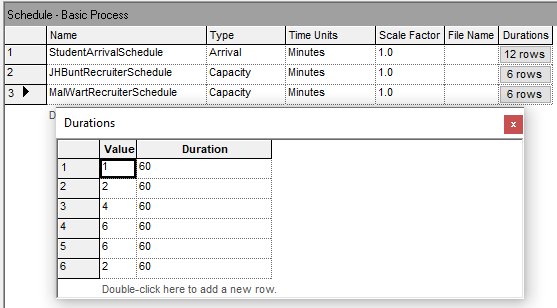
Figure 6.31: Possible resource capacity schedule for STEM Mixer
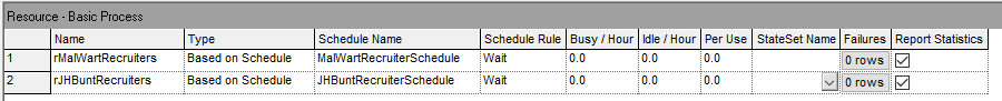
Figure 6.32: Using the resource schedules in the resource module
Figure 6.31 illustrates a possible resource capacity change schedule for the MalMart recruiting station. For simplicity the same schedule will be used for the JHBunt recruiting station. The Arena file for this change can be found in the chapter files as STEM_MixerBothSchedules.doe. Figure 6.32 illustrates how to connect the defined resource schedule to the resource module so that the resource uses the schedule during the simulation. Figure 6.33 and Figure 6.34 present the results when using the resource schedule defined in Figure 6.31.
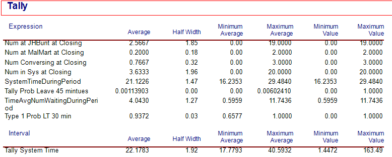
Figure 6.33: Tally results for non-stationary arrivals and time varying resource capacity
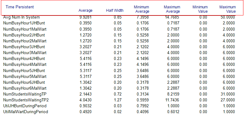
Figure 6.34: =Time persistent results for non-stationary arrivals and time varying resource capacity
The first thing to notice is in Figure 6.33 the substantial drop in overall system time from the near 52 minutes down to about 22 minutes. Also, from Figure 6.34, we see that the utilization of the JHBunt recruiting station is still a bit high (90%) during the peak arrival period. Thus, it may be worth exploring the addition of an additional recruiter during hour 5. We leave the further exploration of this model to the interested reader.
Non-stationary arrival patterns are a fact of life in many systems that handle people. The natural daily processes of waking up, working, etc. all contribute to processes that depend on time. This section illustrated how to model non-stationary arrival processes and illustrated some of the concepts necessary when developing staffing plans for such systems. Incorporating these modeling issues into your simulation models allows for more realistic analysis; however, this also necessitates much more complex statistical analysis of the input distributions and requires careful capture of meaningful statistics. Capturing statistics by time periods is especially important because the statistical results that do not account for the time varying nature of the performance measures may mask what may be actually happening within the model. The overall average across the entire simulation time horizon may be significantly different than what occurs during individual periods of time that correspond to non-stationary situations. A good design must reflect these variations due to time.
In the next section, we continue the exploration of advanced process modeling techniques by illustrating how to model the balking and reneging of entities within queues.