2.6 Modeling a Simple Discrete-Event Dynamic System
This section presents how to model a system in which the state changes at discrete events in time as discussed in the previous section.
2.6.1 A Drive through Pharmacy
This example considers a small pharmacy that has a single line for waiting customers and only one pharmacist. Assume that customers arrive at a drive through pharmacy window according to a Poisson distribution with a mean of 10 per hour. The time that it takes the pharmacist to serve the customer is random and data has indicated that the time is well modeled with an exponential distribution with a mean of 3 minutes. Customers who arrive to the pharmacy are served in the order of arrival and enough space is available within the parking area of the adjacent grocery store to accommodate any waiting customers.
The drive through pharmacy system can be conceptualized as a single server waiting line system, where the server is the pharmacist. An idealized representation of this system is shown in Figure 2.28. If the pharmacist is busy serving a customer, then additional customers will wait in line. In such a situation, management might be interested in how long customers wait in line, before being served by the pharmacist. In addition, management might want to predict if the number of waiting cars will be large. Finally, they might want to estimate the utilization of the pharmacist in order to ensure that the pharmacist is not too busy.
Figure 2.28: Simple drive through pharmacy
2.6.2 Modeling the System
Process modeling is predicated on modeling the process flow of "entities" through a system. Thus, the first question to ask is: What is the system? In this situation, the system is the pharmacist and the potential customers as idealized in Figure 2.28. Now you should consider the entities of the system. An entity is a conceptual thing of importance that flows through a system potentially using the resources of the system. Therefore, one of the first questions to ask when developing a model is: What are the entities? In this situation, the entities are the customers that need to use the pharmacy. This is because customers are discrete things that enter the system, flow through the system, and then depart the system.
Since entities often use things as they flow through the system, a natural question is to ask: What are the resources that are used by the entities? A resource is something that is used by the entities and that may constrain the flow of the entities within the system. Another way to think of resources is to think of the things that provide service in the system. In this situation, the entities “use” the pharmacist in order to get their medicine. Thus, the pharmacist can be modeled as a resource.
Since we are modeling the process flows of the entities through a system, it is natural to ask: What are the process flows? In answering this question, it is conceptually useful to pretend that you are an entity and to ask: What to I do? In this situation, you can pretend that you are a pharmacy customer. What does a customer do? Arrive, get served, and leave. As you can see, initial modeling involves identifying the elements of the system and what those elements do. The next step in building a simulation model is to enhance your conceptual understanding of the system through conceptual modeling. For this simple system, very useful conceptual model has already been given in Figure 2.28. As you proceed through this text, you will learn other conceptual model building techniques. From the conceptual modeling, you might proceed to more logical modeling in preparation for using . A useful logical modeling tool is to develop pseudo-code for the situation. Here is some potential pseudo-code for this situation.
Create customers according to Poisson arrival process
Process the customers through the pharmacy
Dispose of the customers as they leave the system
The pseudo-code represents the logical flow of an entity (customer) through the drive through pharmacy: Arrive (create), get served (process), leave (dispose).
Another useful conceptual modeling tool is the activity diagram. An activity is an operation that takes time to complete. An activity is associated with the state of an object over an interval of time. Activities are defined by the occurrence of two events which represent the activity’s beginning time and ending time and mark the entrance and exit of the state associated with the activity. An activity diagram is a pictorial representation of the process (steps of activities) for an entity and its interaction with resources while within the system. If the entity is a temporary entity (i.e. it flows through the system) the activity diagram is called an activity flow diagram. If the entity is permanent (i.e. it remains in the system throughout its life) the activity diagram is called an activity cycle diagram. The notation of an activity diagram is very simple, and can be augmented as needed to explain additional concepts:
- Queues
shown as a circle with queue labeled inside
- Activities
shown as a rectangle with appropriate label inside
- Resources
shown as small circles with resource labeled inside
- Lines/arcs
indicating flow (precedence ordering) for engagement of entities in activities or for obtaining resources. Dotted lines are used to indicate the seizing and releasing of resources.
- zigzag lines
indicate the creation or destruction of entities
Activity diagrams are especially useful for illustrating how entities interact with resources. Activity diagrams are easy to build by hand and serve as a useful communication mechanism. Since they have a simple set of symbols, it is easy to use an activity diagram to communicate with people who have little simulation background. Activity diagrams are an excellent mechanism to document your conceptual model of the system before building the model in .
Figure 2.29: Activity diagram for drive through pharmacy
Figure 2.29 shows the activity diagram for the pharmacy situation. This diagram was built using Visio software and the drawing is available with the supplemental files for this chapter. You can use this drawing to copy and paste from, in order to form other activity diagrams, but I recommend just drawing activity diagrams free-hand.
An activity diagram describes the life of an entity within the system. The zigzag lines at the top of the diagram indicate the creation of an entity. While not necessary, the diagram has been augmented with like pseudo-code to represent the CREATE statement. Consider following the life of the customer through the pharmacy. Following the direction of the arrows, the customers are first created and then enter the queue. Notice that the diagram clearly shows that there is a queue for the drive-through customers. You should think of the entity flowing through the diagram. As it flows through the queue, the customer attempts to start an activity. In this case, the activity requires a resource. The pharmacist is shown as a resource (circle) next to the rectangle that represents the service activity.
The customer requires the resource in order to start its service activity. This is indicated by the dashed arrow from the pharmacist (resource) to the top of the service activity rectangle. If the customer does not get the resource, they wait in the queue. Once they receive the number of units of the resource requested, they proceed with the activity. The activity represents a delay of time and in this case the resource is used throughout the delay. After the activity is completed, the customer releases the pharmacist (resource). This is indicated by another dashed arrow, with the direction indicating that the resource is "being put back" or released. After the customer completes its service activity, the customer leaves the system. This is indicated with the zigzag lines going to no-where and augmented with the keyword DISPOSE. The dashed arrows of a typical activity diagram have also been augmented with the like pseudo-code of SEIZE and RELEASE. The conceptual model of this system can be summarized as follows:
- System
The system has a pharmacist that acts as a resource, customers that act as entities, and a queue to hold the waiting customers. The state of the system includes the number of customers in the system, in the queue, and in service.
- Events
Arrivals of customers to the system, which occur within an inter-event time that is exponentially distributed with a mean of 6 minutes.
- Activities
The service time of the customers are exponentially distributed with a mean of 3 minutes.
- Conditional delays
A conditional delay occurs when an entity has to wait for a condition to occur in order to proceed. In this system, the customer may have to wait in a queue until the pharmacist becomes available.
With an activity diagram and pseudo-code such as this available to represent a solid conceptual understanding of the system, you can begin the model development process.
Figure 2.30: Overview of pharmacy model
2.6.3 Pharmacy Model Implementation
Now, you are ready to implement the conceptual model. If you haven’t already done so, open up the Arena Environment. Using the Basic Process Panel template, drag the CREATE, PROCESS, and DISPOSE modules into the model window and make sure that they are connected as shown in Figure 2.30. In order to drag and drop the modules, simply select the module within the Basic Process template and drag the module into the model window, letting go of the mouse when you have positioned the module in the desired location. If the module within the model window is highlighted (selected), the next dragged module will automatically be connected. If you placed the modules and they weren’t automatically connected, then you can use the connect toolbar icon. Select the icon and then select the “from" module near the connection exit point and then holding the mouse button down drag to form a connection line to the entry point of the”to" module. The names of the modules will not match what is shown in the figure. You will name the modules as you fill out their dialog boxes.
2.6.4 Specify the Arrival Process
Within Arena nothing happens unless entities enter the model. This is done through the use of the CREATE module. Actually, this statement is not quite true and not quite false. You don’t necessarily have to have a CREATE module in the model to get things to happen, but this requires the use of advanced techniques that are beyond the scope of this book. In the current example, pharmacy customers arrive according to a Poisson process with a mean of \(\lambda\) = 10 per hour. According to probability theory, this implies that the time between arrivals is exponentially distributed with a mean of (\(1/\lambda\)). Thus, for this situation, the mean time between arrivals is 6 minutes.
\[\begin{equation} \frac{1}{\lambda} = \frac{\text{1 hour}}{\text{10 customers}} \times \frac{\text{60 minutes}}{\text{1 hour}} = \frac{\text{6 minutes}}{\text{customer}} \tag{2.6} \end{equation}\]
Open up the CREATE module (by double clicking on it) and fill it in as shown in Figure 2.31. The distribution for the “Time Between Arrivals” is by default Exponential, Random (expo) in the figure. In this instance, the “Value" textbox refers to the mean time between arrivals.”Entities per Arrival" specifies how many customers arrive at each arrival. Since more than one customer does not arrive at a time, the value is set to 1. “Max Arrivals” specifies the total number of arrival events that will occur for the CREATE module. This is set at the default “Infinite” since a fixed number of customers to arrive is not specified for this example. The “First Creation” specifies the time of the first arrival event. Technically, the time to the first event for a Poisson arrival process is exponentially distributed. Hence, expo(6) has been used with the appropriate mean time, where expo(mean) is a function within that generates random variables according to the exponential distribution function with the supplied mean.
Figure 2.31: Pharmacy model CREATE module
Make sure that you specify the units for time as minutes and be sure to press OK; otherwise, your work within the module will be lost. In addition, as you build models you never know what could go wrong; therefore, you should save your models often as you proceed through the model building process. Take the opportunity to save your model before proceeding.
Before proceeding there is one last thing that you should do related to the entities. Since the customers drive cars, you will change the picture associated with the customer entity that was defined in the CREATE module. To do this you will use the ENTITY module within the Basic Process panel. The ENTITY module is a data module. A data module cannot be dragged and dropped into the model window. Data modules require the model builder to enter information in either the spreadsheet window or in a dialog box. To see the dialog box, select the row from the spreadsheet view, right-click and choose the edit via dialog option. You will use the spreadsheet view here. Select the ENTITY module in the Basic Process panel and use the corresponding spreadsheet view to select the picture for the entity as shown in Figure 2.32.
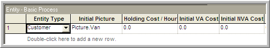
Figure 2.32: Pharmacy model ENTITY module
2.6.5 Specifying the Resources
Go to the Basic Process Panel and select the RESOURCE module. This module is also a data module. As you selected the RESOURCE module, the data sheet window (Figure 2.33) should have changed to reflect this selection. Double-click on the row in the spreadsheet module for the RESOURCE module to add a resource to the model.
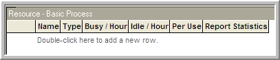
Figure 2.33: RESOURCE module in data sheet view
After the resource row has been added, select the row and right-click. This will bring up a context menu. From this context menu, select edit via dialog box. Make the resulting dialog box look like Figure 2.34 You can also type in the same information that you typed in the dialog box from within the spreadsheet view. This defines a resource that can be used in the model. The resource’s name is Pharmacist and it has a capacity of one. Now, you have to indicate how the customers will use this resource within a process.
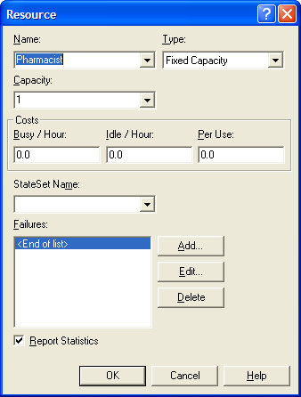
Figure 2.34: RESOURCE dialog box
2.6.6 Specify the Process
A process can be thought of as a set of activities experienced by an entity. There are two basic ways in which processing can occur: resource constrained and resource unconstrained. In the current situation, because there is only one pharmacist and the customer will need to wait if the pharmacist is busy, the situation is resource constrained. A PROCESS module provides for the basic modeling of processes within an model. You specify this within a PROCESS module by having the entity seize the resource for the specified usage time. After the usage time has elapsed, you specify that the resource is released. The basic pseudo-code can now be modified to capture this concept as illustrated in the following pseudo-code.
CREATE customers with EXPO(6) time between arrivals
SEIZE 1 pharmacist
DELAY for EXPO(3) minutes
RELEASE 1 pharmacist
DISPOSE customer
Open up the PROCESS module and fill it out as indicated in Figure 1.23. Change the “Action” drop down dialog box to the (Seize, Delay, Release) option. Use the “Add” button within the “Resources” area to indicate which resources the customer will use. In the pop up Resources dialog, indicate the name of the resource and the number of units desired by the customer. Within the “Delay Type” area, choose Expression as the type of delay and type in expo(3) as the expression. This indicates that the delay, which represents the service time, will be randomly distributed according to an exponential distribution with a mean of 3 minutes. Make sure to change the units accordingly. When a PROCESS module uses the (Seize, Delay, Release) option, Arena automatically translates this to individual SEIZE, DELAY, and RELEASE modules, just like outlined in the pseudo-code. These modules (SEIZE, DELAY, RELEASE) are executed individually as the entities experience the process. It is very useful to understand what happens when these modules are executed.
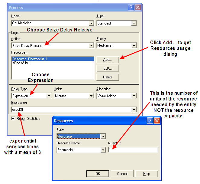
Figure 2.35: PROCESS module seize, delay, release option
When an entity seizes a resource, the number of units available of the resource’s capacity is (automatically) checked against the amount of units requested by the entity. There is a global variable (function) defined for each resource called, NR(Resource ID), that returns the number of units of the resource that have been allocated to entity requests. For example, suppose a resource called, rBankTeller, has capacity, 3, and one of the 3 units (tellers) has already been allocated to a customer for use. That is, one of the tellers is currently serving a customer. In this case, NR(rBankTeller), will have the value 1. There is also a global variable (function) called MR(Resource ID) that holds the number of units of capacity defined for the resource. In this example, MR(rBankTeller) has the value 3. In the drive through pharmacy example the value of MR() is 1. Again, MR() holds the current capacity of the resource. Obviously, resources can have capacity value of various amounts.
The number of available units of the resource is always the difference, MR(Resource ID) - NR(Resource ID). In this bank example, the value of MR(rBankTeller) - NR(rBankTeller) is currently 2 (3 - 1 = 2) because a customer is in service. Thus, an arriving customer that wants one teller will not have to wait in the queue associated with the SEIZE module and will be immediately allocated one of the available tellers. The value of NR(rBankTeller) will be incremented by 1 unit and the number of available units, MR(rBankTeller) - NR(rBankTeller), will decrease by 1. If an entity requests more than the current number of available units of the resource, the entity will be automatically placed in the queue associated with the SEIZE module.
The units of a resource that have been allocated to an entity by a successful SEIZE will remain allocated to that entity until those units are released via a RELEASE module. An entity can release 1 or more units of the allocated resource when executing a RELEASE module. When an entity executes a RELEASE module the allocated units of the resource are given back to the resource and NR(Resource ID) is decremented by the amount released. When the units of the resource are released, the queue associated with the seize (with the highest seize priority) is checked to see if any entities are waiting and if so, those entities are processed to check if their number of units requested of the resource can be allocated. The processing of the queue is based on the queue processing rule (e.g. FIFO (first in, first out), LIFO (last in, first out), random, and priority ranking).
Suppose that a resource has capacity of 1 unit. If there are 2 processes (or seizes) that seize the same resource and entities are waiting in separate queues, the entity that activated the seize with the highest priority will get the resource first. If both seize requests have the same priority, then the entity that activated its seize first will go first (first come first served). The priority field for the seize controls the priority of the seize. It can be anything that evaluates to a number. A resource is considered busy if at least 1 unit of its capacity has been allocated. A resource is considered idle when all units are idle and the resource is not failed or inactive. The failed and inactive states of resources are discussed in Section 6.2.
A common misunderstanding by novice modelers is to think that they must continually check MR(Resource ID) - NR(Resource ID) to see if the resource is available. Do not think this way. The purpose of the SEIZE and RELEASE constructs is to manage the allocation and deallocation of resource units. While there can be legitimate reasons for using the values of NR(Resource ID) and MR(Resource ID) within a model, you should not make the mistake of polling resources for availability. The resource allocation process is done automatically using SEIZE and RELEASE. If you do not like how the resource units are being allocated, then you should use more advanced concepts as discussed in Chapter 6.
Now we are ready to specify how to execute the pharmacy model.
2.6.7 Specify Run Parameters
Let’s assume that the pharmacy is open 24 hours a day, 7 days a week. In other words, it is always open. In addition, assume that the arrival process does not vary with respect to time. Finally, assume that management is interested in understanding the long term behavior of this system in terms of the average waiting time of customers, the average number of customers, and the utilization of the pharmacist. This kind of simulation is called an infinite horizon simulation and will be discussed in more detail in Chapter 5.
To simulate this situation over time, you must specify how long to run the model. Ideally, since management is interested in long run performance, you should run the model for an infinite amount of time to get long term performance; however, you probably don’t want to wait that long! For the sake of simplicity, assume that 10,000 hours of operation is long enough. Within the environment, go to the Run menu item and choose Setup. After the Setup dialog box appears, select the Replication parameters tab and fill it out as shown in Figure 2.36. The Replication Length text box specifies how long the simulation will run. Notice that the base time units were changed to minutes. This ensures that information reported by the model is converted to minutes in the output reports.
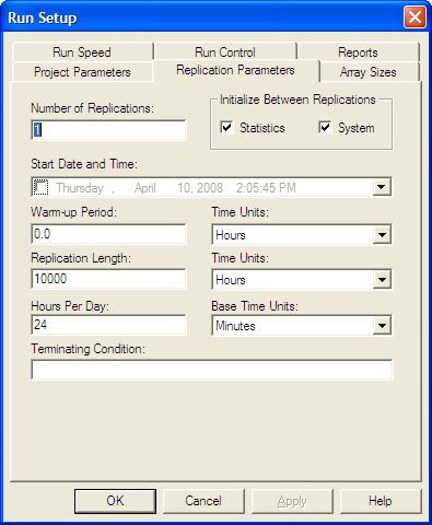
Figure 2.36: Run setup replication parameters tab
The fully completed model is available within this chapter’s files as file, PharmacyModel.doe.
Now, the model is ready to be executed. You can use the Run menu to do this or you can use the convenient "VCR" like run toolbar (Figure 2.37). The Run button causes the simulation to run until the stopping condition is met. The Fast Forward button runs the simulation without animation until the stopping condition is met. The Pause button suspends the simulation run. The Start Over button stops the run and starts the simulation again. The Stop button causes the simulation to stop. The animation slider causes the animation to slow down (to the left) or speed up (to the right).
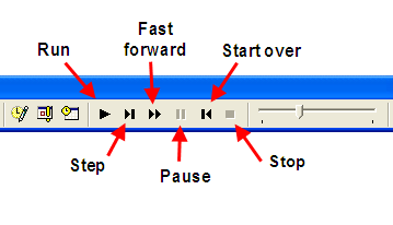
Figure 2.37: Run toolbar
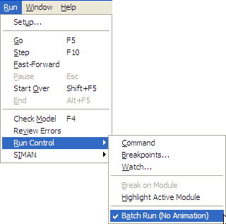
Figure 2.38: Batch run no animation option
When you run the model, you will see the animation related to the customers waiting in line. Because the length of this run is very long, you should use the fast forward button on the "VCR" run toolbar to execute the model to completion without the animation. Instead of using the fast forward button, you can significantly speed up the execution of your model by running the model in batch mode without animation. To do this, you can use the Run menu as shown in Figure 2.38 and then when you use the VCR Run button the model will run much faster without animation.
2.6.8 Analyze the Results
After running the model, you will see a dialog (Figure 2.39) indicating that the simulation run is completed and that the simulation results are ready. Answer yes to open up the report viewer.
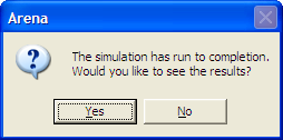
Figure 2.39: Run completion dialog
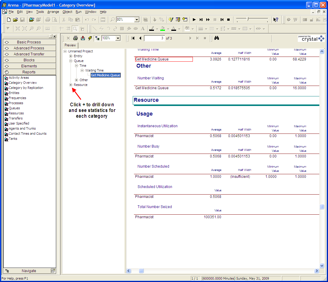
Figure 2.40: Results for pharmacy model
In the reports preview area, you can drill down to see the statistics that you need. Go ahead and do this so that you have the report window as indicated in Figure 2.40. The reports indicate that customers wait about 3 minutes on average in the line. reports the average of the waiting times in the queue as well as the associated 95% confidence interval half-width. In addition, reports the minimum and maximum of the observed values. These results indicate that the maximum a customer waited to get service was 16 minutes. The utilization of the pharmacist is about 50%. This means that about 50% of the time the pharmacist was busy. For this type of system, this is probably not a bad utilization, considering that the pharmacist probably has other in-store duties. The reports also indicate that there was less than one customer on average waiting for service. Using the Reports panel in the Project Bar you can also select specific reports.
also produces a text-based version of these reports in the directory associated with the model. Within the Windows File Explorer, select the modelname.out file, see Figure 1.30. This file can be read with any text editor such as Notepad, see Figure 2.41.
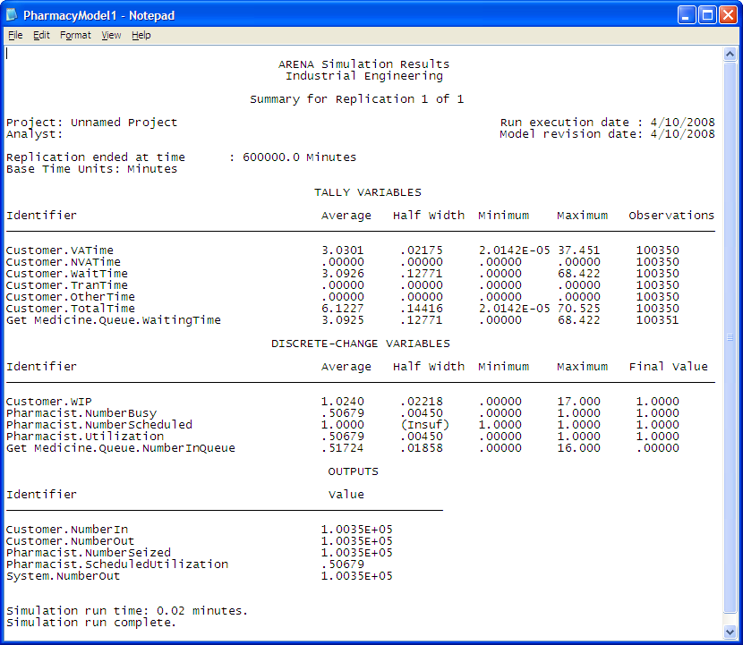
Figure 2.41: Text file summary results
Also as indicated in Figure 2.42, Arena generates additional files when you run the model. The modelname.accdb file is a Microsoft Access database that holds the information displayed by the report writer. The modelname.p file is generated when the model is checked or run. If you have errors or warnings when you check your model, the error file will also show up in the directory of your modelname.doe file
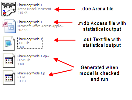
Figure 2.42: Files generated when running Arena
This single server waiting line system is a very common situation in practice. In fact, this exact situation has been studied mathematically through a branch of operations research called queuing theory. As will be covered in Appendix C for specific modeling situations, formulas for the long term performance of queuing systems can be derived. This particular pharmacy model happens to be an example of an M/M/1 queuing model. The first M stands for Markov arrivals, the second M stands for Markov service times, and the 1 represents a single server. Markov was a famous mathematician who examined the exponential distribution and its properties. According to queuing theory, the expected number of customer in queue, \(L_q\), for the M/M/1 model is:
\[\begin{equation} \begin{aligned} L_q & = \dfrac{\rho^2}{1 - \rho} \\ \rho & = \lambda/\mu \\ \lambda & = \text{arrival rate to queue} \\ \mu & = \text{service rate} \end{aligned} \tag{2.7} \end{equation}\]
In addition, the expected waiting time in queue is given by \(W_q = L_q/\lambda\). In the pharmacy model, \(\lambda\) = 1/6, i.e. 1 customer every 6 minutes on average, and \(\mu\) = 1/3, i.e. 1 customer every 3 minutes on average. The quantity, \(\rho\), is called the utilization of the server. Using these values in the formulas for \(L_q\) and \(W_q\) results in:
\[ \begin{aligned} \rho & = 0.5 \\ L_q & = \dfrac{0.5 \times 0.5}{1 - 0.5} = 0.5 \\ W_q & = \dfrac{0.5}{1/6} = 3 \: \text{minutes} \end{aligned} \]
In comparing these analytical results with the simulation results, you can see that they match to within statistical error. Later in this text, the analytical treatment of queues and the simulation of queues will be developed. These analytical results are available for this special case because the arrival and service distributions are exponential; however, simple analytical results are not available for many common distributions, e.g. lognormal. With simulation, you can easily estimate the above quantities as well as many other performance measures of interest for wide ranging queuing situations. For example, through simulation you can easily estimate the chance that there are 3 or more cars waiting.