8.1 Analyzing Multiple Systems
The analysis of multiple systems stems from a number of objectives. First, you may want to perform a sensitivity analysis on the simulation model. In a sensitivity analysis, you want to measure the effect of small changes to key input parameters to the simulation. For example, you might have assumed a particular arrival rate of customers to the system and want to examine what would happen if the arrival rate decreased or increased by 10%. Sensitivity analysis can help you to understand how robust the model is to variations in assumptions. When you perform a sensitivity analysis, there may be a number of factors that need to be examined in combination with other factors. This may result in a large number of experiments to run. This section discusses how to use the Process Analyzer to analyze multiple experiments. Besides performing a sensitivity analysis, you may want to compare the performance of multiple alternatives in order to choose the best alternative. This type of analysis is performed using multiple comparison statistical techniques. This section will also illustrate how to perform a multiple comparison with the best analysis using the Process Analyzer.
8.1.1 Sensitivity Analysis Using the Process Analyzer
For illustrative purposes, a sensitivity analysis on the LOTR Makers Inc. system will be performed. Suppose that you were concerned about the effect of various factors on the operation of the newly proposed system and that you wanted to understand what happens if these factors vary from the assumed values. In particular, the effects of the following factors in combination with each other are of interest:
Number of sales calls made each day: What if the number of calls made each day was 10% higher or lower than its current value?
Standard deviation of inner ring diameter: What if the standard deviation was reduced or increased by 2% compared to its current value?
Standard deviation of outer ring diameter: What if the standard deviation was reduced or increased by 2% compared to its current value?
The resulting factors and their levels are given in Table 8.1.
| Factor | Description | Base Level | % Change | Low Level | High Level |
|---|---|---|---|---|---|
| A | # sales calls per day | 100 | \(\pm\) 10 % | 90 | 110 |
| B | Std. Dev. of outer ring diameter | 0.005 | \(\pm\) 2 % | 0.0049 | 0.0051 |
| C | Std. Dev. of inner ring diameter | 0.002 | \(\pm\) 2 % | 0.00196 | 0.00204 |
The Process Analyzer allows the setting up and the batch running of multiple experiments. With the Process Analyzer, you can control certain input parameters (variables, resource capacities, replication parameters) and define specific response variables (COUNTERS, DSTATS (time-persistent statistics), TALLY (tally based statistics), OUTPUT statistics) for a given simulation model. An important aspect of using the Process Analyzer is to plan the development of the model so that you can have access to the items that you want to control.
In the current example, the factors that need to vary have already been specified as variables; however the Process Analyzer has a 4 decimal place limit on control values. Thus, for specifying the standard deviations for the rings a little creativity is required. Since the actual levels are simply a percentage of the base level, you can specify the percent change as the level of the factor and multiply accordingly in the model. For example, for factor (C) the standard deviation of the inner ring, you can specify 0.98 as the low value since \(0.98 \times 0.002 = 0.00196\).
Table 8.2 shows the resulting experimental scenarios
in terms of the multiplying factor. Within the model, you need to ensure
that the variables are multiplied. For example, define three new
variables vNCF, vIDF, and vODF to represent the multiplying factors and
multiply the original variables where ever they are used:
In Done Calling? DECIDE module:
vNumCalls*vNCFIn Determine Diameters ASSIGN module:
NORM(vIDM, vIDS*vIDF, vStream)In Determine Diameters ASSIGN module:
NORM(vODM, vODS*vODF, vStream)
Another approach to achieving this would be to define an EXPRESSION and
use the expression within the model. For example, you can define an
expression eNumCalls = vNumCalls*vNCF and use eNumCalls within the
model. The advantage of this is that you do not have to hunt throughout
the model for all the changes. The definitions can be easily located
within the EXPRESSION module.
| Scenario | vNCF (A) | vIDF (B) | vODF (C) |
|---|---|---|---|
| 1 | 0.90 | 0.98 | 0.98 |
| 2 | 0.90 | 0.98 | 1.02 |
| 3 | 0.90 | 1.02 | 0.98 |
| 4 | 0.90 | 1.02 | 1.02 |
| 5 | 1.1 | 0.98 | 0.98 |
| 6 | 1.1 | 0.98 | 1.02 |
| 7 | 1.1 | 1.02 | 0.98 |
| 8 | 1.1 | 1.02 | 1.02 |
The Process Analyzer is a separate program that is installed when the Environment is installed. Since it is a separate program, it has its own help system, which you can access after starting the program. You can access the Process Analyzer through your Start Menu or through the Tools menu within the Environment. The first thing to do after starting the Process Analyzer is to start a new PAN file via the File \(>\) New menu. You should then see a screen similar to Figure 8.1.
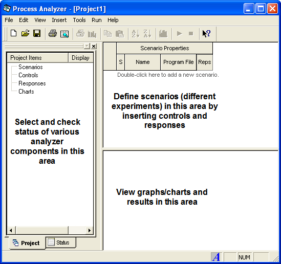
Figure 8.1: The Process Analyzer
In the Process Analyzer you define the scenarios that you want to be executed. A scenario consists of a model in the form of a (.p) file, a set of controls, and a set of responses. To generate a (.p) file, you can use Run \(>\) Check Model. If the check is successful, this will create a (.p) file with the same name as your model to be located in the same directory as the model. Each scenario refers to one (.p) file but the set of scenarios can consist of scenarios that have different (.p) files. Thus, you can easily specify models with different structure as part of the set of scenarios.
To start a scenario, double-click on the add new scenario row within the scenario properties area. You can type in the name for the scenario and the name of the (.p) file (or use the file browser) to specify the scenario as shown in Figure 8.2.
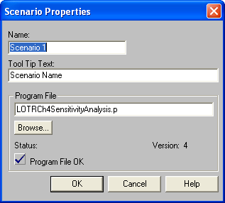
Figure 8.2: Adding a new scenario
Then you can use the Insert menu to
insert controls and response variables for the scenario. The insert
control dialog is shown in Figure 8.3. Using this you should define a
control for NREPS (number of replications), vStream (random number
stream), vNCF (number of sales calls factor), vIDF (standard deviation
of inner ring factor), and vODF (standard deviation of outer ring
factor). For each of the controls, be sure to specify the proper data
type (e.g. vStream is an Integer, vIDF is a real).
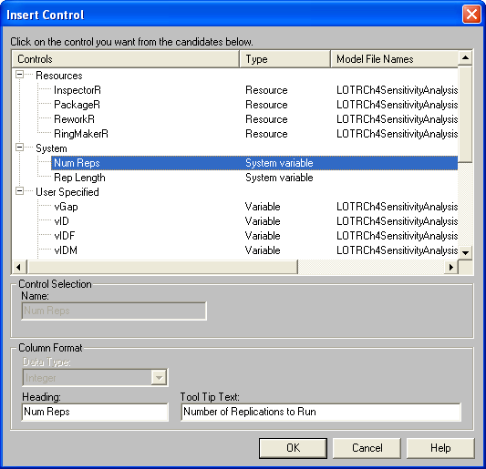
Figure 8.3: Inserting controls
After specifying the first scenario, select the row, right-click and
choose Duplicate Scenario(s) until you have defined 8 scenarios. Then,
you should complete the scenario definitions as shown in
Figure 8.4. To insert a response, use the
Insert menu and select the appropriate responses. In this analysis, you
will focus on the average time it takes a pair of rings to complete
production (PairOfRings.TotalTime), the throughput per day
(Throughput), and the average time spent waiting at the rework station
(Rework.Queue.WaitingTime).
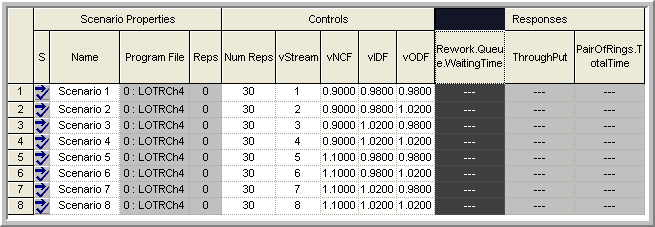
Figure 8.4: Experimental setup controls and responses
Since a different stream number has been specified for each of the scenarios, they will all be independent. Within the context of experimental design, this is useful because traditional experimental design techniques (such as response surface analysis) depend on the assumption that the experimental design points are independent. If you use the same stream number for each of the scenarios then you will be using common random numbers. From the standpoint of the analysis via traditional experimental design techniques this poses an extra complication. The analysis of experimental designs with common random numbers is beyond the scope of this text. The interested reader should refer to (Kleijnen 1988) and (Kleijnen 1998).
To run all the experiments consecutively, select the scenarios that you want to run and use the Run menu or the VCR like run button. Each scenario will run the number of specified replications and the results for the responses will be tabulated in the response area as shown in Figure 8.5. After the simulations have been completed, you can add more responses and the results will be shown.
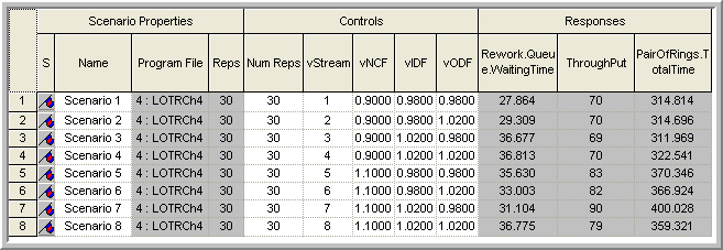
Figure 8.5: Results after running the scenarios
The purpose in performing a sensitivity analysis is two-fold: 1) to see if small changes in the factors result in significant changes in the responses and 2) to check if the expected direction of change in the response is achieved. Intuitively, if there is low variability in the ring diameters, then you should expect less rework and thus less queuing at the rework station. In addition, if there is more variability in the ring diameters then you might expect more queuing at the rework station. From the responses for scenarios 1 and 4, this basic intuition is confirmed. The results in Figure 8.5 indicate that scenario 4 has a slightly higher rework waiting time and that scenario 1 has the lowest rework waiting time. Further analysis can be performed to examine the statistical significance of these differences.
In general, you should examine the other responses to validate that your simulation is performing as expected for small changes in the levels of the factors. If the simulation does not perform as expected, then you should investigate the reasons. A more formal analysis involving experimental design and analysis techniques may be warranted to ensure statistical confidence in your analysis.
Again, within a simulation context, you know that there should be differences in the responses, so that standard ANOVA tests of differences in means are not really meaningful. In other words, they simply tell you whether you took enough samples to detect a difference in the means. Instead, you should be looking at the magnitude and direction of the responses. A full discussion of the techniques of experimental design is beyond the scope of this chapter. For a more detailed presentation of the use of experimental design in simulation, you are referred to (Law 2007) and (Kleijnen 1998).
Selecting a particular response cell will cause additional statistical information concerning the response to appear in the status bar at the left-hand bottom of the Process Analyzer main window. In addition, if you place your cursor in a particular response cell, you can build charts associated with the individual replications associated with that response. Place your cursor in the cell as shown in Figure 8.5 and right-click to insert a chart. The Chart Wizard will start and walk you through the chart building. In this case, you will make a simple bar chart of the rework waiting times for each of the 30 replications of scenario 1. In the chart wizard, select “Compare the replication values of a response for a single scenario” and choose the Column chart type. Proceed through the chart wizard by selecting Next (and then Finish) making sure that the waiting time is your performance measure. You should see a chart similar to that shown in Figure 8.6.
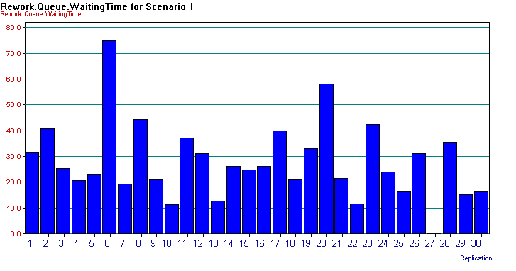
Figure 8.6: Individual scenario chart for rework waiting time
If you right-click on the chart options pop-up menu, you can gain access to the data and properties of the chart (Figure 8.7). From this dialog you can copy the data associated with the chart. This gives you an easy mechanism for cutting and pasting the data into another application for additional analysis.
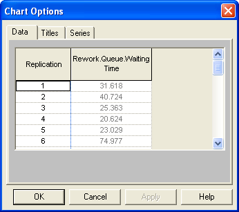
Figure 8.7: Data within chart options
To create a chart across the scenarios, select the column associated with the desired response and right-click. Then, select Insert Chart from the pop up menu. This will bring up the chart wizard with the “Compare the average values of a response across scenarios” option selected. In this example, you will make a box and whisker chart of the waiting times. Follow the wizard through the process until you have created a chart as shown in Figure 8.8.
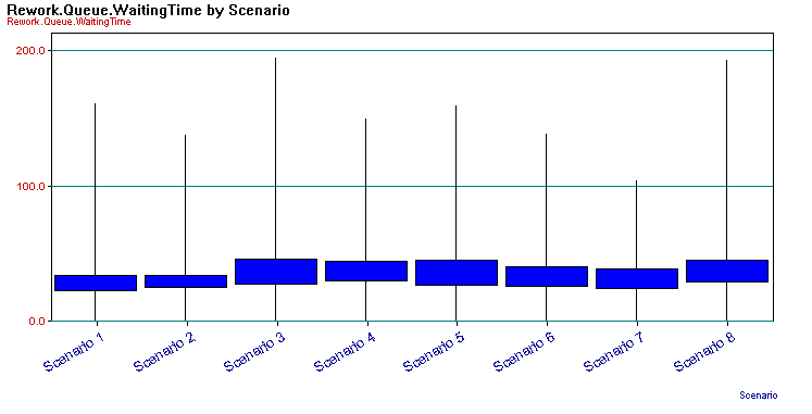
Figure 8.8: Box-Whiskers chart across scenarios
There are varying definitions of what constitutes a box-whiskers plot. In the Process Analyzer, the box-whiskers plot shows whiskers (narrow thin lines) to the minimum and maximum of the data and a box (dark solid rectangle) which encapsulates the inter-quartile range for the data (\(3^{rd} \, \text{Quartile} – 1^{st} \, \text{Quartile}\)). Fifty percent of the data is within the box. This plot can give you an easy way to compare the distribution of the responses across the scenarios. Right-clicking on the chart give you access to the data used to build the chart, and in particular it includes the 95% half-widths for confidence intervals on the responses. Table 8.3 shows the data copied from the box-whiskers chart.
| Scenario | Min (A) | Max | Low | Hi | 95% CI |
|---|---|---|---|---|---|
| Scenario 1 | 0 | 160.8 | 22.31 | 33.42 | 5.553 |
| Scenario 2 | 0 | 137.2 | 24.93 | 33.69 | 4.382 |
| Scenario 3 | 0 | 194.1 | 27.47 | 45.88 | 9.205 |
| Scenario 4 | 0 | 149.8 | 29.69 | 43.93 | 7.12 |
| Scenario 5 | 0 | 159.2 | 26.58 | 44.68 | 9.052 |
| Scenario 6 | 0 | 138.3 | 26.11 | 39.9 | 6.895 |
| Scenario 7 | 0 | 103.5 | 24 | 38.2 | 7.101 |
| Scenario 8 | 0 | 193.1 | 28.82 | 44.73 | 7.956 |
This section illustrated how to setup experiments to test the sensitivity of various factors within your models by using the Process Analyzer. After you are satisfied that your simulation model is working as expected, you often want to use the model to help to pick the best design out of a set of alternatives. The case of two alternatives has already been discussed; however, when there are more than two alternatives, more sophisticated statistical techniques are required in order to ensure that a certain level of confidence in the decision making process is maintained. The next section overviews why more sophisticated techniques are needed. In addition, the section illustrates how to facilitate the analysis using the Process Analyzer.
8.1.2 Multiple Comparisons with the Best
Suppose that you are interested in analyzing \(k\) systems based on performance measures \(\theta_i, \, i = 1,2, \ldots, k\). The goals may be to compare each of the \(k\) systems with a base case (or existing system), to develop an ordering among the systems, or to select the best system. In any case, assume that some decision will be made based on the analysis and that the risk associated with making a bad decision needs to be controlled. In order to perform an analysis, each \(\theta_i\) must be estimated, which results in sampling error for each individual estimate of \(\theta_i\). The decision will be based upon all the estimates of \(\theta_i\) (for every system). The the sampling error involves the sampling for each configuration. This compounds the risk associated with an overall decision. To see this more formally, the “curse” of the Bonferroni inequality needs to be understood.
The Bonferroni inequality states that given a set of (not necessarily independent) events, \(E_i\), which occur with probability, \(1-\alpha_i\), for \(i = 1,2,\ldots, k\) then a lower bound on the probability of the intersection of the events is given by:
\[P \lbrace \cap_{i=1}^k E_i \rbrace \geq 1 - \sum_{i=1}^k \alpha_i\]
In words, the Bonferroni inequality states that the probability of all the events occurring is at least one minus the sum of the probability of the individual events occurring. This inequality can be applied to confidence intervals, which are probability statements concerning the chance that the true parameter falls within intervals formed by the procedure.
Suppose that you have \(c\) confidence intervals each with confidence \(1-\alpha_i\). The \(i^{th}\) confidence interval is a statement \(S_i\) that the confidence interval procedure will result in an interval that contains the parameter being estimated. The confidence interval procedure forms intervals such that \(S_i\) will be true with probability \(1-\alpha_i\). If you define events, \(E_i = \lbrace S_i \text{is true}\rbrace\), then the intersection of the events can be interpreted as the event representing all the statements being true.
\[P\lbrace \text{all} \, S_i \, \text{true}\rbrace = P \lbrace \cap_{i=1}^k E_i \rbrace \geq 1 - \sum_{i=1}^k \alpha_i = 1 - \alpha_E\]
where \(\alpha_E = \sum_{i=1}^k \alpha_i\). The value \(\alpha_E\) is called the overall error probability. This statement can be restated in terms of its complement event as:
\[P\lbrace \text{one or more} \, S_i \, \text{are false} \rbrace \leq \alpha_E\]
This gives an upper bound on the probability of a false conclusion based on the confidence intervals.
This inequality can be applied to the use of confidence intervals when comparing multiple systems. For example, suppose that you have, \(c = 10\), 90% confidence intervals to interpret. Thus, \(\alpha_i = 0.10\), so that
\[\alpha_E = \sum_{i=1}^{10} \alpha_i = \sum_{i=1}^{10} (0.1) = 1.0\]
Thus, \(P\lbrace \text{all} \, S_i \, \text{true}\rbrace \geq 0\) or \(P\lbrace\text{one or more} \, S_i \, \text{are false} \rbrace \leq 1\). In words, this is implying that the chance that all the confidence intervals procedures result in confidence intervals that cover the true parameter is greater than zero and less than 1. Think of it this way: If your boss asked you how confident you were in your decision, you would have to say that your confidence is somewhere between zero and one. This would not be very reassuring to your boss (or for your job!).
To combat the “curse” of Bonferroni, you can adjust your confidence levels in the individual confidence statements in order to obtain a desired overall risk. For example, suppose that you wanted an overall confidence of 95% on making a correct decision based on the confidence intervals. That is you desire, \(\alpha_E\) = 0.05. You can pre-specify the \(\alpha_i\) for each individual confidence interval to whatever values you want provided that you get an overall error probability of \(\alpha_E = 0.05\). The simplest approach is to assume \(\alpha_i = \alpha\). That is, use a common confidence level for all the confidence intervals. The question then becomes: What should \(\alpha\) be to get \(\alpha_E\) = 0.05? Assuming that you have \(c\) confidence intervals, this yields:
\[\alpha_E = \sum_{i=1}^c \alpha_i = \sum_{i=1}^c \alpha = c\alpha\]
So that you should set \(\alpha = \alpha_E/c\). For the case of \(\alpha_E = 0.05\) and \(c = 10\), this implies that \(\alpha = 0.005\). What does this do to the width of the individual confidence intervals? Since the \(\alpha_i = \alpha\) have gotten smaller, the confidence coefficient (e.g. \(z\) value or \(t\) value) used in confidence interval will be larger, resulting in a wider confidence interval. Thus, you must trade-off your overall decision error against wider (less precise) individual confidence intervals.
Because the Bonferroni inequality does not assume independent events it can be used for the case of comparing multiple systems when common random numbers are used. In the case of independent sampling for the systems, you can do better than simply bounding the error. For the case of comparing \(k\) systems based on independent sampling the overall confidence is:
\[P \lbrace \text{all}\, S_i \, \text{true}\rbrace = \prod_{i=1}^c (1 - \alpha_i)\]
If you are comparing \(k\) systems where one of the systems is the standard (e.g. base case, existing system, etc.), you can reduce the number of confidence intervals by analyzing the difference between the other systems and the standard. That is, suppose system one is the base case, then you can form confidence intervals on \(\theta_1 - \theta_i\) for \(i = 2,3,\ldots, k\). Since there are \(k - 1\) differences, there are \(c = k - 1\) confidence intervals to compare.
If you are interested in developing an ordering between all the systems, then one approach is to make all the pair wise comparisons between the systems. That is, construct confidence intervals on \(\theta_j - \theta_i\) for \(i \neq j\). The number of confidence intervals in this situation is
\[c = \binom{k}{2} = \frac{k(k - 1)}{2}\]
The trade-off between overall error probability and the width of the individual confidence intervals will become severe in this case for most practical situations.
Because of this problem a number of techniques have been developed to allow the selection of the best system (or the ranking of the systems) and still guarantee an overall pre-specified confidence in the decision. The Process Analyzer uses a method based on multiple comparison procedures as described in (Goldsman and Nelson 1998) and the references therein. See also (Law 2007) for how these methods relate to other ranking and selection methods.
While it is beyond the scope of this textbook to review multiple comparison with the best (MCB) procedures, it is useful to have a basic understanding of the form of the confidence interval constructed by these procedures. To see how MCB procedures avoid part of the issues with having a large number of confidence intervals, we can note that the confidence interval is based on the difference between the best and the best of the rest. Suppose we have \(k\) system configurations to compare and suppose that somehow you knew that the \(i^{th}\) system is the best. Now, consider a confidence interval system’s \(i\) performance metric, \(\theta_i\), of the following form:
\[ \theta_i - \max_{j \neq i} \theta_j \] This difference is the difference between the best (\(\theta_i\)) and the second best. This is because if \(\theta_i\) is the best, when we find the maximum of those remaining, it will be next best (i.e. second best). Now, let us suppose that system \(i\) is not the best. Reconsider, \(\theta_i - \max_{j \neq i} \theta_j\). Then, this difference will represent the difference between system \(i\), which is not the best, and the best of the remaining systems. In this case, because \(i\) is not the best, the set of systems considered in \(\max_{j \neq i} \theta_j\) will contain the best. Therefore, in either case, this difference:
\[ \theta_i - \max_{j \neq i} \theta_j \] tells us exactly what we want to know. This difference allows us to compare the best system with the rest of the best. MCB procedures build \(k\) confidence intervals:
\[ \theta_i - \max_{j \neq i} \theta_j \ \text{for} \ i=1,2, \dots,k \] Therefore, only \(k\) confidence intervals need to be considered to determine the best rather than, \(\binom{k}{2}\).
This form of confidence interval has also been combined with the concept of an indifference zone. Indifference zone procedures use a parameter \(\delta\) that indicates that the decision maker is indifferent between the performance of two systems, if the difference is less than \(\delta\). This indicates that even if there is a difference, the difference is not practically significant to the decision maker within this context. These procedures attempt to ensure that the overall probability of correct selection of the best is \(1-\alpha\), whenever, \(\theta_{i^{*}} - \max_{j \neq i^{*}} \theta_j > \delta\), where \(i^{*}\) is the best system and \(\delta\) is the indifference parameter. This assumes that larger is better in the decision making context. There are a number of single stage and multiple stage procedures that have been developed to facilitate decision making in this context.
One additional item of note to consider when using these procedures. The results may not be able to distinguish between the best and others. For example, assuming that we desire the maximum (bigger is better), then let \(\hat{i}\) be the index of the system found to be the largest and let \(\hat{\theta}_{i}\) be the estimated performance for system \(i\), then, these procedures allow the following:
- If \(\hat{\theta}_{i} - \hat{\theta}_{\hat{i}} + \delta \leq 0\), then we declare that system \(i\) not the best.
- If \(\hat{\theta}_{i} - \hat{\theta}_{\hat{i}} + \delta > 0\), then we can declare that system \(i\) is not statistically different from the best. In this case, system \(i\), may in fact be the best.
The procedure used by Arena’s Process Analyzer allows for the opportunity to provide an indifference parameter and the procedure will highlight via color which systems are best or not statistically different from the best. The statistical software, \(R\), also has a package that facilitates multiple comparison procedures called multcomp. The interested reader can refer to the references for the package for further details.
Using the scenarios that were already defined within the sensitivity analysis section, the following example illustrates how you can select the best system with an overall confidence of 95%. The procedure built into the Process Analyzer can handle common random numbers. The previously described scenarios were set up and re-executed as shown in Figure 8.9. Notice in the figure that the stream number for each scenario was set to the same value, thereby, applying common random numbers. The PAN file for this analysis is called LOTR-MCB.pan and can be found in the supporting files folder called SensitivityAnalysis for this chapter.
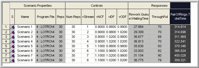
Figure 8.9: Results for MCB analysis using common random numbers
Suppose you want to pick the best scenario in terms of the average time that a pair of rings spends in the system. Furthermore, suppose that you are indifferent between the systems if they are within 5 minutes of each other. Thus, the goal is to pick the system that has the smallest time with 95% confidences.
To perform this analysis, right-click on the PairOfRings.TotalTime
response column and choose insert chart. Make sure that you have
selected “Compare the average values of a response across scenarios” and
select a suitable chart in the first wizard step. This example uses a
Hi-Lo chart which displays the confidence intervals for each response as
well has the minimum and maximum value of each response. The comparison
procedure is available with the other charts as well. On the second
wizard step, you can pick the response that you want
(PairOfRings.TotalTime) and choose next. On the 3rd wizard step you
can adjust your titles for your chart. When you get to the 4th wizard
step, you have the option of identifying the best scenario.
Figure 8.10 illustrates the settings for the
current situation. Select the “identify the best scenarios option” with
the smaller is better option, and specify an indifference amount (Error
tolerance) as 5 minutes. Using the Show Best Scenarios button, you can
see the best scenarios listed. Clicking Finish causes the chart to be
created and the best scenarios to be identified in red (scenarios 1, 2,
3, & 4) as shown in Figure 8.11.
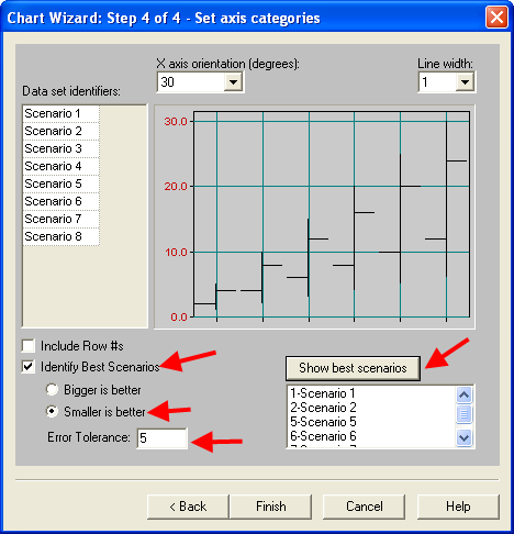
Figure 8.10: Identifying the best scenario
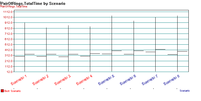
Figure 8.11: Possible best scenarios
As indicated in Figure 8.11, four possible scenarios have been recommended as the best. This means that you can be 95% confident that any of these 4 scenarios is the best based on the 5 minute error tolerance. This analysis has narrowed down the set of scenarios, but has not recommended a specific scenario because of the variability and closeness of the responses. To further narrow the set of possible best scenarios down, you can run additional replications of the identified scenarios and adjust your error tolerance. Thus, with the Process Analyzer you can easily screen systems out of further consideration and adjust your statistical analysis in order to meet the objectives of your simulation study.
Now that we have a good understanding of how to effectively use the Process Analyzer, we will study how to apply these concepts on an Arena Contest problem.