4.9 Exercises
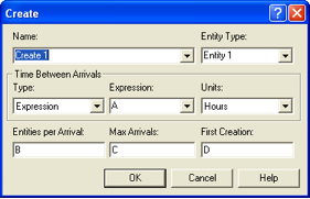
Figure 4.107: CREATE Module
Specify expressions for A, B, C, and D in the above CREATE module to properly generate customers for the T-Shirt Stand.
A: \(\underline{\hspace{3cm}}\)
B: \(\underline{\hspace{3cm}}\)
C: \(\underline{\hspace{3cm}}\)
D: \(\underline{\hspace{3cm}}\)
Exercise 4.6 TV sets arrive at a two-inspector station for testing. The time between arrivals is exponential with a mean of 15 minutes. The inspection time per TV set is exponential with a mean of 10 minutes. On the average, 82 percent of the sets pass inspection. The remaining 18% are routed to an adjustment station with a single operator. Adjustment time per TV set is uniform between 7 and 14 minutes. After adjustments are made, sets are routed back to the inspection station to be retested. We are interested in estimating the total time a TV set spends in the system before it is released.
Develop a model for this situation. Report the average system time for the TV sets based on 20 replications of 4800 minutes. Also report statistics for the average number of times a given TV is adjusted.Exercise 4.7 A simple manufacturing system is staffed by 3 operators. Parts arrive according to a Poisson process with a mean rate of 2 per minute to a workstation for a drilling process at one of three identical drill presses. The parts wait in a single queue until a drill press is available. Each part has a particular number of holes that need to be drilled. Each hole takes a Lognormal time to be drilled with an approximate mean of 1 minute and a standard deviation of 30 seconds. Once the holes are drilled, the part goes to the grinding operation. At the grinding operation, one of the 3 available operators grinds out the burrs on the part. This activity takes approximately 5 minutes plus or minus 30 seconds. After the grinding operation the part leaves the system.
Develop model for this situation. Report the average system time for the parts based on 20 replications of 4800 minutes.Exercise 4.8 The Hog BBQ Joint is interested in understanding the flow of customers for diner (5 pm to 9 pm). Customers arrive in parties of 2, 3, 4, or 5 with probabilities 0.4, 0.3, 0.2, 0.1, respectively. The time between arrivals is exponentially distributed with a mean of 1.4 minutes. Customers must arrive prior to 9 pm in order to be seated. The dining area has 50 tables. Each table can seat 2 people. For parties, with more than 2 customers, the tables are moved together. Each arriving group gets in line to be seated. If there are already 6 parties in line, the arriving group will leave and go to another restaurant. The time that it takes to be served is triangularly distributed with parameters (14, 19, 24) in minutes. The time that it takes to eat is lognormally distributed with a mean of 24 minutes and a standard deviation of 5 minutes. When customers are finished eating, they go to the cashier to pay their bill. The time that it takes the cashier to process the customers is gamma distributed with a mean of 1.5 minutes and a standard deviation of 0.5 minutes.
Develop an model for this situation. Simulate 30 days of operation. Make a table like the following to summarize your results.| Average | Half-width | |
|---|---|---|
| Number of customers served | ||
| Number of busy tables | ||
| Number of waiting parties | ||
| Number of parties that depart without eating | ||
| Utilization of cashier | ||
| Customer System Time (in minutes) | ||
| Probability of waiting to be seated \(>\) 5 minutes |
Exercise 4.11 Hungry customers arrive to a Mickey R’s drive through restaurant at a mean rate of 10 per hour according to a Poisson process. Management is interested in improving the total time spent within the system (i.e. from arrival to departure with their food).
Management is considering a proposed system that splits the order taking, payment activity and the order delivery processes. The first worker will take the orders from an order-taking speaker. This takes on average 1 minute plus or minus 20 seconds uniformly distributed. When the order taking activity is completed, the making of the order will start. It takes approximately 3 minutes (plus or minus 20 seconds) to make the customer’s order, uniformly distributed. Meanwhile, the customer will be instructed to drive to the first window to pay for the order. Assume that the time that it takes the customer to move forward is negligible. The first worker accepts the payment from the customer. This takes on average 45 seconds plus or minus 20 seconds uniformly distributed. After paying for the order the customer is instructed to pull forward to the second window, where a second worker delivers the order. Assume that the time that it takes the customer to move forward is negligible.
If the order is not completed by the time the customer reaches the second window, then the customer must wait for the order to be completed. If the order is completed before the customer arrives to the 2nd window, then the order must wait for the customer. After both the order and the customer are at the 2nd window, the 2nd worker packages the customer’s order and gives it to the customer. This takes approximately 30 seconds with a standard deviation of 10 seconds, lognormally distributed. After the customer receives their order they depart.
Simulate this system for the period from 10 am to 2 pm. Report the total time spent in the system for the customers based on 30 days.Exercise 4.12 The city is considering improving its hazardous waste and bulk item drop off area to improve service. Cars arrive to the drop off area at a rate of 10 per hour according to a Poisson process. Each car contains items for drop off. There is a 10% chance that the car will contain 1 item, a 50% chance that the car will contain 2 items, and a 40% chance that the car will contain 3 items. There is an 80% chance that an item will be hazardous (e.g. chemicals, light bulbs, electronic equipment, etc.) and a 20% chance that the item will be a bulk item, which cannot be picked up in the curbside recycling program. Of the 80% of items that have hazardous waste, about 10% are for electronic equipment that must be inspected and taken apart.
A single worker assists the citizen in taking the material out of their car and moving the material to the recycling center. This typically takes between 0.5 to 1.5 minutes per item (uniformly distributed) if the item is not a bulk item. If the item is a bulk item, then the time takes a minimum of 1 minute, most likely 2.5 minutes, with a maximum of 4 minutes per item triangularly distributed. The worker finishes all items in a car before processing the next car.
Another worker will begin sorting the items immediately after the item is unloaded. This process takes 1-2 minutes per item uniformly distributed. If the item is electronic equipment, the items are placed in front of a special disassembly station to be taken apart.
The same worker that performs sorting also performs the disassembly of the electronic parts. Items that require sorting take priority over items that require disassembly. Each electronic item takes between 8 to 16 minutes uniformly distributed to disassemble.
The hazardous waste recycling center is open for 7 hours per day, 5 days per week. Simulate 12 weeks of performance and estimate the following quantities:Utilization of the workers
Average waiting time for items waiting to be unloaded
Average number of items waiting to be unloaded
Average number of items waiting to be sorted
Average waiting time of items to be sorted
Average number of items waiting to be disassembled
Average waiting time for items waiting to be disassembled.
Exercise 4.13 Orders for street lighting poles require the production of the tapered pole, the base assembly, and the wiring/lighting assembly package. Orders are released to the shop floor with an exponential time between arrival of 20 minutes. Assume that all the materials for the order are already available within the shop floor.
Once the order arrives, the production of the pole begins. Pole production requires that the sheet metal be cut to a trapezoidal shape. This process takes place on a cutting shear. After cutting, the pole is rolled using a press brake machine. This machine rolls the sheet to an almost closed form. After rolling, the pole is sealed on an automated welding machine. Each of these processes are uniformly distributed with ranges \([3, 5]\), \([6,10]\), and \([4,8]\) minutes respectively.
While the pole is being produced, the base is being prepared. The base is a square metal plate with four holes drilled for bolting the place to the mounting piece and a large circular hole for attaching the pole to the base. The base plates are in stock so that only the holes need to be cut. This is done on a water jet cutting machine. This process takes approximately 20 minutes plus or minus 2 minutes, triangularly distributed. After the holes are cut, the plate goes to a grinding/deburring station, which takes between 10 minutes, exponentially distributed.
Once the plate and the pole are completed, they are transported to the inspection station. Inspection takes 20 minutes, exponentially distributed with 1 operator. There could be a quality problem with the pole or with the base (or both). The chance that the problem is with the base is 0.02 and the chance that the problem is with the pole is 0.01. If either or both have a quality issue, the pole and base go to a rework station for rework. Rework is performed by a single operator and typically takes between 100 minutes, exponentially distributed. After rework, the pole and base are sent to final assembly. If no problems occur with the pole or the base, the pole and base are sent directly to final assembly.
At the assembly station, the pole is fixed to the base plate and the wiring assembly is placed within the pole. This process takes 1 operator approximately 30 minutes with a standard deviation of 4 minutes according to a lognormal distribution. After assembly, the pole is sent to the shipping area for final delivery.
The shop is interested in taking on additional orders which would essentially double the arrival rate. Estimate the utilization of each resource and the average system time to produce an order for a lighting pole. Assume that the system runs 5 days per week, with two, eight hours shifts per day. Any production that is not completed within 5 days is continued on the next available shift. Run the model for 10 years assuming 52 weeks per year to report your results.Exercise 4.14 Patients arrive at an emergency room where they are treated and then depart. Arrivals are exponentially distributed with a mean time between arrivals of 0.3 hours. Upon arrival, patients are assigned a rating of 1 to 5, depending on the severity of their ailments. Patients in Category 1 are the most severe, and they are immediately sent to a bed where they await medical attention. All other patients must first wait in the receiving room until a basic registration form and medical record are completed. They then proceed to a bed.
The emergency room has three beds, one registration nurse, and two doctors. In all cases, the priority for allocating these resources is based on the severity of the ailment. Hint: Read the help for the QUEUE module and rank the queue by the severity attribute. The registration time for patients in Categories 2 through 5 is Uniform (0.1, 0.2) hours. The treatment time for all patients is triangularly distributed with the minimum, most likely, and maximum values differing according to the patient’s category. The distribution of patients by category and the corresponding minimum, most likely, and maximum treatment times are summarized below.
| Category | 1 | 2 | 3 | 4 | 5 |
|---|---|---|---|---|---|
| Percent | 6 | 8 | 18 | 33 | 35 |
| Minimum | 0.8 | 0.7 | 0.4 | 0.2 | 0.1 |
| Most Likely | 1.2 | 0.95 | 0.6 | 0.45 | 0.35 |
| Maximum | 1.6 | 1.1 | 0.75 | 0.6 | 0.45 |
The required responses for this simulation include:
Average number of patients waiting for registration
Utilization of beds
System time of each type of patient and overall (across patient types)
Using a run length of 30 days, develop a model to estimate the required responses. Report the responses based on estimating the system time of a patient regardless of type based on 50 replications.
| Type | Percentage | Cooking Time |
|---|---|---|
| 1 | 30% | Uniform(0.3,0.8) |
| 2 | 15% | Uniform(0.8,1.1) |
| 3 | 55% | Uniform(1.0, 1.4) |
Use stream 2 for the ordering distribution, stream 3 for the paying distribution, streams 4, 5 and 6, for the type 1, 2, and 3 cooking distributions, respectively. Use stream 7 for the distribution across the order types.
Model the system for 8 hours of operation with 30 replications. Make a table like the following to summarize your answers for your replications.
| Average | Half-width | |
|---|---|---|
| Type 1 Throughput | ||
| Type 2 Throughput | ||
| Type 3 Throughput | ||
| Utilization of cashiers | ||
| Utilization of cooks | ||
| Customer System Time (in minutes) | ||
| Customer Waiting Time (in minutes) | ||
| Probability of wait \(>\) 5 minutes |
Exercise 4.20 Jobs arrive in batches of ten items each. The inter-arrival time is EXPO(2) hours. The machine shop contains 2 milling machines and one drill press. About 30% of the items require drilling before being processed on the milling machine. Drilling time per item is UNIF(10, 15) minutes. The milling time is EXPO(15) minutes for items that do not require drilling, and UNIF(15,20) for items that do. Assume that the shop has two 8-hour shifts each day and that you are only interested in the first shift’s performance. Any jobs left over at the end of the first shift are left to be processed by the second shift. Estimate the average number of jobs left for the second shift to complete at the end of the first shift to within plus or minus 5 jobs with 95% confidence. What is your replication length? Number of replications? Determine the utilization of the drill press and the milling machines as well as the average time an item spends in the system.
The average system time of items that pass inspection on the first attempt. Measure this quantity such that you are 95% confident to within +/- 3 minutes.
The average number of jobs completed per week.
Sketch an activity diagram for this situation.
Assume that there are 2 technicians at the repair station, 1 inspector at the inspection station, and 1 technician at the disassembly station. Develop a model for this situation.
Assume that there are 2 technicians at the repair station and 1 inspector at the inspection station. The disassembly station is also staffed by the 2 technicians that are assigned to the repair station. Develop a model for this situation.
Exercise 4.22 As part of a diabetes prevention program, a clinic is considering setting up a screening service in a local mall. They are considering two designs: Design A: After waiting in a single line, each walk-in patient is served by one of three available nurses. Each nurse has their own booth, where the patient is first asked some medical health questions, then the patient’s blood pressure and vitals are taken, finally, a glucose test is performed to check for diabetes. In this design, each nurse performs the tasks in sequence for the patient. If the glucose test indicates a chance of diabetes, the patient is sent to a separate clerk to schedule a follow-up at the clinic. If the test is not positive, then the patient departs.
Design B: After waiting in a single line, each walk-in is served in order by a clerk who takes the patient’s health information, a nurse who takes the patient’s blood pressure and vitals, and another nurse who performs the diabetes test. If the glucose test indicates a chance of diabetes, the patient is sent to a separate clerk to schedule a follow-up at the clinic. If the test is not positive, then the patient departs. In this configuration, there is no room for the patient to wait between the tasks; therefore, a patient who as had their health information taken cannot move ahead unless the nurse taking the vital signs is available. Also, a patient having their glucose tested must leave that station before the patient in blood pressure and vital checking can move ahead.
Patients arrive to the system according to a Poisson arrival process at a rate of 9.5 per hour (stream 1). Assume that there is a 5% chance (stream 2) that the glucose test will be positive. For design A, the time that it takes to have the paperwork completed, the vitals taken, and the glucose tested are all log-normally distributed with means of 6.5, 6.0, and 5.5 minutes respectively (streams 3, 4, 5). They all have a standard deviation of approximately 0.5 minutes. For design B, because of the specialization of the tasks, it is expected that the mean of the task times will decrease by 10%.
Assume that the clinic is open from 10 am to 8 pm (10 hours each day) and that any patients in the clinic before 8 pm are still served. The distribution used to model the time that it takes to schedule a follow up visit is a WEIB(2.6, 7.3) distribution using stream 6.
Make a statistically valid recommendation as to the best design based on the average system time of the patients. We want to be 95% confident of our recommendation to within 2 minutes.
Exercise 4.23 A copy center has one fast copier and one slow copier. The copy time per page for the fast copier is thought to be lognormally distributed with a mean of 1.6 seconds and a standard deviation of 0.3 seconds. A co-op Industrial Engineering student has collected some time study data on the time to copy a page for the slow copier. The times, in seconds, are given in the data set associated with Exercise B.13.
The copy times for the slow and fast copiers are given on a per page basis. Thus, the total time to perform a copy job of N pages is the sum of the copy times for the N individual pages. Each individual page’s time is random.
Customers arrive to the copy center according to a Poisson process with a mean rate of 1 customer every 40 seconds. The number of copies requested by each customer is equally likely over the range of 10 and 50 copies. The customer is responsible for filling out a form that indicates the number of copies to be made. This results in a copy job which is processed by the copying machines in the copy center. The copying machines work on the entire job at one time.
The policy for selecting a copier is as follows: If the number of copies requested is less than or equal to 30, the slow copier will be used. If the number of copies exceeds 30, the fast copier will be used, with one exception: If no jobs are in queue on the slow copier and the number of jobs waiting for the fast copier is at least two, then the customer will be served by the slow copier. After the customer gives the originals for copying, the customer proceeds to the service counter to pay for the copying. Assume that giving the originals for copying requires no time and thus does not require action by the copy center personnel. In addition, assume that one cashier handles the payment counter only so that sufficient workers are available to run the copy machines. The time to complete the payment transaction is lognormally distributed with a mean of 20 seconds and a standard deviation of 10 seconds. As soon as both the payment and the copying job are finished, the customer takes the copies and departs the copying center. The copy center starts out a day with no customers and is open for 10 hours per day.
Management has requested that the co-op Industrial Engineer develop a model because they are concerned that customers have to wait too long for copies. Recently, several customers complained about long waits. Their standard is that the probability that a customer waits longer than 4 minutes should be no more than 10%. They define a customer’s waiting time as the time interval from when the customer enters the store to the time the customer leaves the store with their completed copy job. If the waiting time criteria is not met, several options are available: The policy for allocating jobs to the fast copier could be modified or the company could purchase an additional copier which could be either a slow copier or a fast copier.
Develop a model for this problem. Based on 25 replications, report in table form, the appropriate statistics on the waiting time of customers, the daily throughput of the copy center, and the utilization of the payment clerk. In addition estimate the probability that a customer spends in the system is longer than 4 minutes.Exercise 4.24 Passengers arrive at an airline terminal according to an exponential distribution for the time between arrivals with a mean of 1.5 minutes (stream 1). Of the arriving passengers 7% are frequent flyers (stream 2). The time that it takes the passenger to walk from the main entrance to the check-in counter is uniform between 2.5 and 3.5 minutes (stream 3). Once at the counter the travellers must wait in a single line until one of four agents is available to serve them. The check-in time (in minutes) is Gamma distributed with a mean of 5 minutes and a standard deviation of 4 minutes (stream 4). When their check-in is completed, passengers with carry-on only go directly to security. Those with a bag to check, walk to another counter to drop their bag. The time to walk to bag check is uniform(1,2) minutes (stream 9). Since the majority of the flyers are business, only 25% of the travellers have a bag to check (stream 5). At the baggage check, there is a single line served by one agent. The time to drop off the bag at the bag check stations is lognormally distributed with a mean of 2 minutes and a standard deviation of 1 minute (stream 6). After dropping off their bags, the traveller goes to security. The time to walk to security (either after bag check or directly from the check in counter) is exponentially distributed with a mean of 8 minutes (stream 10). At the security check point, there is a single line, served by two TSA agents. The TSA agents check the boarding passes of the passengers. The time that it takes to check the boarding pass is triangularly distributed with parameters (2, 3, 4) minutes (stream 7). After getting their identity checked, the travellers go through the screening process. We are not interested in the screening process. However, the time that it takes to get through screening is distributed according to a triangular distribution with parameters (5, 7, 9) minutes (stream 8). After screening, the walking time to the passenger’s gate is exponentially distributed with a mean of 5 minutes (stream 11).
We are interested in estimating the average time it takes from arriving at the terminal until a passenger gets to their gate. This should be measured overall and by type (frequent flyer versus non-frequent flyer).
Assume that the system should be studied for 16 hours per day.
- Report the average and 95% confidence interval half-width on the following based on the simulation of 10 days of operation. Report all time units in minutes.
| Statistic | Average | Half-Width |
|---|---|---|
| Utilization of the check-in agents | ||
| Utilization of the TSA agents | ||
| Utilization of the Bag Check agent | ||
| Frequent Flyer Total time to Gate | ||
| Non-Frequent Flyer Total time to Gate | ||
| Total time to Gate regardless of type | ||
| Number of travellers in the system | ||
| Number of travellers waiting for check-in | ||
| Number of travellers waiting for security | ||
| Time spent waiting for check-in | ||
| Time spent waiting for security |
- Based on the results of part (a) determine the number of replications necessary to estimate the total time to reach their gate regardless of type to within \(\pm\) 1 minute with 95% confidence.
| Test Plan | % of parts | Sequence |
|---|---|---|
| 1 | 20% | 2,3,2,1 |
| 2 | 12.5% | 3,1 |
| 3 | 37.5% | 1,3,1 |
| 4 | 20% | 2,3 |
| 5 | 10% | 2,1,3 |
| Test Plan | Testing Time Parameters | Repair Time Parameters |
|---|---|---|
| 1 | (20,4.1), (12,4.2), (18,4.3), (16,4.0) | (30,60,80) |
| 2 | (12,4), (15,4) | (45,55,70) |
| 3 | (18,4.2), (14,4.4), (12,4.3) | (30,40,60) |
| 4 | (24,4), (30,4) | (35,65,75) |
| 5 | (20,4.1), (15,4), (12,4.2) | (20,30,40) |
Management is interested in understanding where the potential bottlenecks are in the system and in developing alternatives to mitigate those bottlenecks so that they can still handle the contract. The new contract stipulates that 80% of the time the testing and repairs should be completed within 480 minutes. The company runs 2 shifts each day for each 5 day work week. Any jobs not completed at the end of the second shift are carried over to first shift of the next working day. Assume that the contract is going to last for 1 year (52 weeks). Build a simulation model that can assist the company in assessing the risks associated with the new contract.
Exercise 4.26 Parts arrive at a 4 workstation system according to an exponential inter-arrival distribution with a mean of 10 minutes. The workstation A has 2 machines. The three workstations (B, C, D) each have a single machine. There are 3 part types, each with an equal probability of arriving. The process plan for the part types are given below. The entries are for exponential distributions with the mean processing time (MPT) parameter given.
| Workstation, MPT | Workstation, MPT | Workstation, MPT |
| A, 9.5 | C, 14.1 | B, 15 |
| A, 13.5 | B, 15 | C, 8.5 |
| A, 12.6 | B, 11.4 | D, 9.0 |
Assume that the transfer time between arrival and the first station, between all stations, and between the last station and the system exit is 3 minutes.Using the ROUTE, SEQUENCE, and STATION modules, simulate the system for 30000 minutes and discuss the potential bottlenecks in the system.