5.2 Statistical Analysis Techniques for Warmup Detection
There are two basic methods for performing infinite horizon simulations. The first is to perform multiple replications. This approach addresses independence and normality in a similar fashion as the finite horizon case, but special procedures will be needed to address the non-stationary aspects of the data. The second basic approach is to work with one very long replication. Both of these methods depend on first addressing the problem of the non-stationary aspects of the data. The next section looks at ways to mitigate the non-stationary aspect of within-replication data for infinite horizon simulations.
5.2.1 Assessing the Effect of Initial Conditions
Consider the output stochastic process \(X_i\) of the simulation. Let \(F_i(x|I)\) be the conditional cumulative distribution function of \(X_i\) where \(I\) represents the initial conditions used to start the simulation at time 0. If \(F_i(x|I) \rightarrow F(x)\) when \(i \rightarrow \infty\), for all initial conditions \(I\), then \(F(x)\) is called the steady state distribution of the output process. (Law 2007).
In infinite horizon simulations, estimating parameters of the steady state distribution, \(F(x)\), such as the steady state mean, \(\theta\), is often the key objective. The fundamental difficulty associated with estimating steady state performance is that unless the system is initialized using the steady state distribution (which is not known), there is no way to directly observe the steady state distribution.
It is true that if the steady state distribution exists and you run the simulation long enough the estimators will tend to converge to the desired quantities. Thus, within the infinite horizon simulation context, you must decide on how long to run the simulations and how to handle the effect of the initial conditions on the estimates of performance. The initial conditions of a simulation represent the state of the system when the simulation is started. For example, in simulating the pharmacy system, the simulation was started with no customers in service or in the line. This is referred to as empty and idle. The initial conditions of the simulation affect the rate of convergence of estimators of steady state performance.
Because the distributions \(F_i(x|I)\) at the start of the replication tend to depend more heavily upon the initial conditions, estimators of steady state performance such as the sample average, \(\bar{X}\), will tend to be biased. A point estimator, \(\hat{\theta}\), is an unbiased estimator of the parameter of interest, \(\theta\), if \(E[\hat{\theta}] = \theta\). That is, if the expected value of the sampling distribution is equal to the parameter of interest then the estimator is said to be unbiased. If the estimator is biased then the difference, \(E[\hat{\theta}] - \theta\), is called the bias of the estimator \(\hat{\theta}\).
Note that any individual difference between the true parameter, \(\theta\), and a particular observation, \(X_i\), is called error, \(\epsilon_i = X_i -\theta\). If the expected value of the errors is not zero, then there is bias. A particular observation is not biased. Bias is a property of the estimator. Bias is analogous to being consistently off target when shooting at a bulls-eye. It is as if the sights on your gun are crooked. In order to estimate the bias of an estimator, you must have multiple observations of the estimator. Suppose that you are estimating the mean waiting time in the queue as per the previous example and that the estimator is based on the first 20 customers. That is, the estimator is:
\[\bar{W}_r = \dfrac{1}{20}\sum_{i=1}^{20} W_{ir}\]
and there are \(r = 1, 2, \ldots 10\) replications. Table 5.1 shows the sample average waiting time for the first 20 customers for 10 different replications. In the table, \(B_r\) is an estimate of the bias for the \(r^{th}\) replication, where \(W_q = 1.6\bar{33}\). Upon averaging across the replications, it can be seen that \(\bar{B}= -0.9536\), which indicates that the estimator based only on the first 20 customers has significant negative bias, i.e. on average it is less than the target value.
| r | \(\bar{W}_r\) | \(B_r = \bar{W}_r - W_q\) |
|---|---|---|
| 1 | 0.194114 | -1.43922 |
| 2 | 0.514809 | -1.11852 |
| 3 | 1.127332 | -0.506 |
| 4 | 0.390004 | -1.24333 |
| 5 | 1.05056 | -0.58277 |
| 6 | 1.604883 | -0.02845 |
| 7 | 0.445822 | -1.18751 |
| 8 | 0.610001 | -1.02333 |
| 9 | 0.52462 | -1.10871 |
| 10 | 0.335311 | -1.29802 |
| \(\bar{\bar{W}}\) = 0.6797 | \(\bar{B}\) = -0.9536 |
This is the so called initialization bias problem in steady state simulation. Unless the initial conditions of the simulation can be generated according to \(F(x)\), which is not known, you must focus on methods that detect and/or mitigate the presence of initialization bias.
One strategy for initialization bias mitigation is to find an index, \(d\), for the output process, \({X_i}\), so that \({X_i; i = d + 1, \ldots}\) will have substantially similar distributional properties as the steady state distribution \(F(x)\). This is called the simulation warm up problem, where \(d\) is called the warm up point, and \({i = 1,\ldots,d}\) is called the warm up period for the simulation. Then the estimators of steady state performance are based only on \({X_i; i = d + 1, \ldots}\).
For example, when estimating the steady state mean waiting time for each replication \(r\) the estimator would be:
\[\bar{W_r} = \dfrac{1}{n-d}\sum_{i=d+1}^{n} W_{ir}\]
For time-based performance measures, such as the average number in queue, a time \(T_w\) can be determined past which the data collection process can begin. Estimators of time-persistent performance such as the sample average are computed as:
\[\bar{Y}_r = \dfrac{1}{T_e - T_w}\int_{T_w}^{T_e} Y_r(t)\mathrm{d}t\]
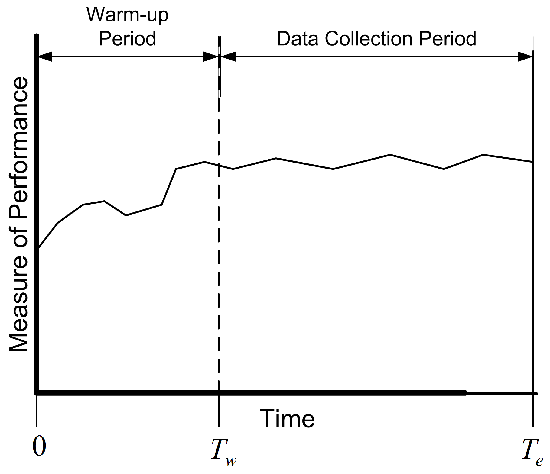
Figure 5.9: The concept of the warm up period
Figure 5.9 show the concept of a warm up period for a simulation replication. When you perform a simulation, you can easily specify a time-based warm up period using the Run \(>\) Setup \(>\) Replication Parameters panel. In fact, even for observation based data, it will be more convenient to specify the warm up period in terms of time. A given value of \(T_w\) implies a particular value of \(d\) and vice a versa. Specifying a warm up period, causes an event to be scheduled for time \(T_w\). At that time, all the accumulated statistical counters are cleared so that the net effect is that statistics are only collected over the period from \(T_w\) to \(T_e\). The problem then becomes that of finding an appropriate warm up period.
Before proceeding with how to assess the length of the warm up period, the concept of steady state needs to be further examined. This subtle concept is often misunderstood or misrepresented. Often you will hear the phrase: The system has reached steady state. The correct interpretation of this phrase is that the distribution of the desired performance measure has reached a point where it is sufficiently similar to the desired steady state distribution. Steady state is a concept involving the performance measures generated by the system as time goes to infinity. However, sometimes this phrase is interpreted incorrectly to mean that the system itself has reached steady state. Let me state emphatically that the system never reaches steady state. If the system itself reached steady state, then by implication it would never change with respect to time. It should be clear that the system continues to evolve with respect to time; otherwise, it would be a very boring system! Thus, it is incorrect to indicate that the system has reached steady state. Because of this, do not to use the phrase: The system has reached steady state.
Understanding this subtle issue raises an interesting implication concerning the notion of deleting data to remove the initialization bias. Suppose that the state of the system at the end of the warm up period, \(T_w\), is exactly the same as at \(T = 0\). For example, it is certainly possible that at time \(T_w\) for a particular replication that the system will be empty and idle. Since the state of the system at \(T_w\) is the same as that of the initial conditions, there will be no effect of deleting the warm up period for this replication. In fact there will be a negative effect, in the sense that data will have been thrown away for no reason. Deletion methods are predicated on the likelihood that the state of the system seen at \(T_w\) is more representative of steady state conditions. At the end of the warm up period, the system can be in any of the possible states of the system. Some states will be more likely than others. If multiple replications are made, then at \(T_w\), each replication will experience a different set of conditions at \(T_w\). Let \(I_{T_w}^r\) be the initial conditions (state) at time \(T_w\) on replication \(r\). By setting a warm up period and performing multiple replications, you are in essence sampling from the distribution governing the state of the system at time \(T_w\). If \(T_w\) is long enough, then on average across the replications, you are more likely to start collecting data when the system in states that are more representative over the long term (rather than just empty and idle).
Many methods and rules have been proposed to determine the warm up period. The interested reader is referred to (Wilson and Pritsker 1978), Lada, Wilson, and Steiger (2003), (Litton and Harmonosky 2002), White, Cobb, and Spratt (2000), Cash et al. (1992), and (Rossetti and Delaney 1995) for an overview of such methods. This discussion will concentrate on the visual method proposed in (Welch 1983) called the Welch Plot.
5.2.2 Using a Welch Plot to Detect the Warmup Period
The basic idea behind Welch’s graphical procedure is simple:
Make \(R\) replications. Typically, \(R \geq 5\) is recommended.
Let \(Y_{rj}\) be the \(j^{th}\) observation on replication \(r\) for \(j = 1,2,\cdots,m_r\) where \(m_r\) is the number of observations in the \(r^{th}\) replication, and \(r = 1,2,\cdots,n\),
Compute the averages across the replications for each \(j = 1, 2, \ldots, m\), where \(m = min(m_r)\) for \(r = 1,2,\cdots,n\).
\[\bar{Y}_{\cdot j} = \dfrac{1}{n}\sum_{r=1}^n Y_{rj}\]
Plot, \(\bar{Y}_{\cdot j}\) for each \(j = 1, 2, \ldots, m\)
Apply smoothing techniques to \(\bar{Y}_{\cdot j}\) for \(j = 1, 2, \ldots, m\)
Visually assess where the plots start to converge
Let’s apply Welch’s procedure to the replications generated from the Lindley equation simulation. Using the 10 replications stored on sheet 10Replications, compute the average across each replication for each customer. In Figure 5.10, cell B2 represents the average across the 10 replications for the \(1^{st}\) customer. Column D represents the cumulative average associated with column B.
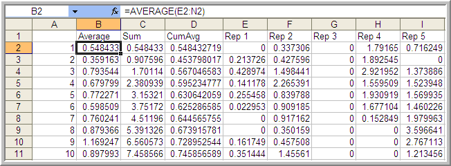
Figure 5.10: Computing the averages for the Welch plot
Figure 5.11 is the plot of the cumulative average (column D) superimposed on the averages across replications (column B). The cumulative average is one method of smoothing the data. From the plot, you can infer that after about customer 3000 the cumulative average has started to converge. Thus, from this analysis you might infer that \(d = 3000\).
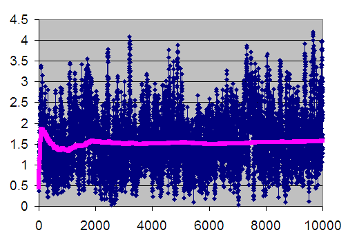
Figure 5.11: Welch plot with superimposed cumulative average Line
When you perform an infinite horizon simulation by specifying a warm up period and making multiple replications, you are using the method of replication-deletion. If the method of replication-deletion with \(d = 3000\) is used for the current example, a slight reduction in the bias can be achieved as indicated in Table 5.2.
| \(r\) | \(\bar{W}_r\) \((d = 0)\) | \(\bar{W}_r(d = 3000)\) | \(B_r(d = 0)\) | \(B_r(d = 3000)\) |
|---|---|---|---|---|
| 1 | 1.594843 | 1.592421 | -0.03849 | -0.04091 |
| 2 | 1.452237 | 1.447396 | -0.1811 | -0.18594 |
| 3 | 1.657355 | 1.768249 | 0.024022 | 0.134915 |
| 4 | 1.503747 | 1.443251 | -0.12959 | -0.19008 |
| 5 | 1.606765 | 1.731306 | -0.02657 | 0.097973 |
| 6 | 1.464981 | 1.559769 | -0.16835 | -0.07356 |
| 7 | 1.621275 | 1.75917 | -0.01206 | 0.125837 |
| 8 | 1.600563 | 1.67868 | -0.03277 | 0.045347 |
| 9 | 1.400995 | 1.450852 | -0.23234 | -0.18248 |
| 10 | 1.833414 | 1.604855 | 0.20008 | -0.02848 |
| \(\bar{\bar{W}}\) = 1.573617 | \(\bar{\bar{W}}\) = 1.603595 | \(\bar{B}\) = -0.05972 | \(\bar{B}\) = -0.02974 | |
| s = 0.1248 | s = 0.1286 | s = 0.1248 | s = 0.1286 | |
| 95% LL | 1.4843 | 1.5116 | -0.149023 | -0.121704 |
| 95% UL | 1.6629 | 1.6959 | -0.029590 | 0.062228 |
While not definitive for this simple example, the results suggest that deleting the warm up period helps to reduce initialization bias. This model’s warm up period will be further analyzed using additional tools available in the next section.
In performing the method of replication-deletion, there is a fundamental trade-off that occurs. Because data is deleted, the variability of the estimator will tend to increase while the bias will tend to decrease. This is a trade-off between a reduction in bias and an increase in variance. That is, accuracy is being traded off against precision when deleting the warm up period. In addition to this trade off, data from each replication is also being thrown away. This takes computational time that could be expended more effectively on collecting usable data. Another disadvantage of performing replication-deletion is that the techniques for assessing the warm up period (especially graphical) may require significant data storage. The Welch plotting procedure requires the saving of data points for post processing after the simulation run. In addition, significant time by the analyst may be required to perform the technique and the technique is subjective.
When a simulation has many performance measures, you may have to perform a warm up period analysis for every performance measure. This is particularly important, since in general, the performance measures of the same model may converge towards steady state conditions at different rates. In this case, the length of the warm up period must be sufficiently long enough to cover all the performance measures. Finally, replication-deletion may simply compound the bias problem if the warm up period is insufficient relative to the length of the simulation. If you have not specified a long enough warm up period, you are potentially compounding the problem for \(n\) replications.
Despite all these disadvantages, replication-deletion is very much used in practice because of the simplicity of the analysis after the warm up period has been determined. Once you are satisfied that you have a good warm up period, the analysis of the results is the same as that of finite horizon simulations. Replication-deletion also facilitates the use of experimental design techniques that rely on replicating design points.
In addition, replication-deletion facilitates the use of such tools as the Process Analyzer and OptQuest. The Process Analyzer and OptQuest will be discussed in Chapter 8. The next section illustrates how to perform the method of replication-deletion on this simple M/M/1 model.