5.3 Performing the Method of Replication-Deletion
The first step in performing the method of replication-deletion is to determine the length of the warm up period. This example illustrates how to:
Save the values from observation and time-based data to files for post processing
Setup and run the multiple replications
Make Welch plots based on the saved data
Interpret the results
The file MM1-ReplicationDeletionCSV.doe contains the M/M/1 model for with the time between arrivals \(exp (E[Y_i] = 1.0)\) and the service times \(exp(E[Y_i] = 0.7)\) set in the CREATE and DELAY modules respectively. Figure 5.12 shows the overall flow of the model. Since the waiting times in the queue need to be captured, an ASSIGN module has been used to mark the time that the customer arrives to the queue. Once the customer exits the SEIZE module they have been removed from the queue to start service. At that point a RECORD module is used to capture the time interval representing the queueing time.
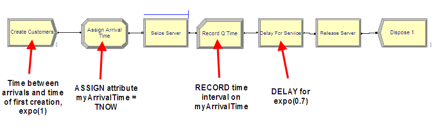
Figure 5.12: MM1 Arena model
Using the STATISTIC data module, the statistics collected within the replications can be captured to files for post processing by the Output Analyzer. This example will collect the queue time of each customer and the number of customers in the queue over time. Figure 5.13 shows how to add a statistic using the STATISTIC data module that will capture observation-based data (e.g. queue time) to a file. The Type of the statistic is Tally and the Tally Name corresponds to the name specified in the RECORD module used to capture the observations. When a name for the output file is specified, the model will store every observation and the time of the observation to a file with the extension (.dat). These files are not human-readable, but can be processed by Arena’s Output Analyzer. However, we have set the extension to (.csv) because we will post process the files using other programs.
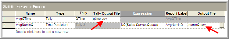
Figure 5.13: STATISTIC Module with CSV extension added
Changing the extension of the output file is not sufficient to change the actual data type of the file that is written. We have set the extension in the STATISTIC module simply to ensure that the file name has the csv extension when saved to a file. Many programs will automatically recognize the CSV extension. In a moment, we will use the Run Setup \(>\) Run Control Advanced Settings (Figure 5.15) tab to ensure that the files are written out as text.
Figure 5.13 also shows how to create a statistic to capture
the number in queue over time to a file. The type of the statistic is
indicated as Time-Persistent and an expression must be given that
represents the value of the quantity to be observed through time. In
this case, the expression builder has been used to select the current
number of entities in the Seize Server.Queue (using the NQ(queue ID)
function). When the Output File is specified, the value of the
expression and the time of the observation are written to a file.
When performing a warm-up period analysis, the first decision to make is the length of each replication. In general, there is very little guidance that can be offered other than to try different run lengths and check for the sensitivity of your results. Within the context of queueing simulations, the work by (Whitt 1989) offers some ideas on specifying the run length, but these results are difficult to translate to general simulation models.
Since the purpose here is to determine the length of the warm up period, then the run length should be bigger than what you suspect the warm up period to be. In this analysis, it is better to be conservative. You should make the run length as long as possible given your time and data storage constraints. Banks et al. (2005) offer the rule of thumb that the run length should be at least 10 times the amount of data deleted. That is, \(n \geq 10d\), where \(d\) is the number of observations deleted from the series. In terms of time, \(T_e \geq 10T_w\), where \(T_w\) is the length of the warm up period in the time units of the simulation. Of course, this is a “catch 22” situation because you need to specify \(n\) or equivalently \(T_e\) in order to assess \(T_w\). Setting \(T_e\) very large is recommended when doing a preliminary assessment of \(T_w\). Then, you can use the rule of thumb of 10 times the amount of data deleted when doing a more serious assessment of \(T_w\) (e.g. using Welch plots etc.)
A preliminary assessment of the current model has already been performed based on the previously described Excel simulation. That assessment suggested a deletion point of at least \(d = 3000\) customers. This can be used as a starting point in the current effort. Now, \(T_w\) needs to be determined based on \(d\). The value of \(d\) represents the customer number for the end of the warm up period. To get \(T_w\), you need to answer the question: How long (on average) will it take for the simulation to generate \(d\) observations. In this model, the mean number of arrivals is 1 customer per minute. Thus, the initial \(T_w\) is
\[3000 \; \text{customers} \times \frac{\text{minute}}{\text{1 customer}} \; = 3000 \; \text{minutes}\]
and therefore the initial \(T_e\) should be 30,000 minutes. Thus, in general, if we let \(\eta\) be the rate of occurrence of the observations, \(\delta = 1/\eta\) be the time between occurrence, and \(d\) the desired number of observations to delete, we have that the length of the warm up period should be:
\[\begin{equation} T_w = \frac{d}{\eta} = d \times \delta \tag{5.1} \end{equation}\]
Specify 30,000 minutes for the replication length and 10 replications on the Run \(>\) Setup \(>\) Replication Parameters as shown in Figure 5.14.
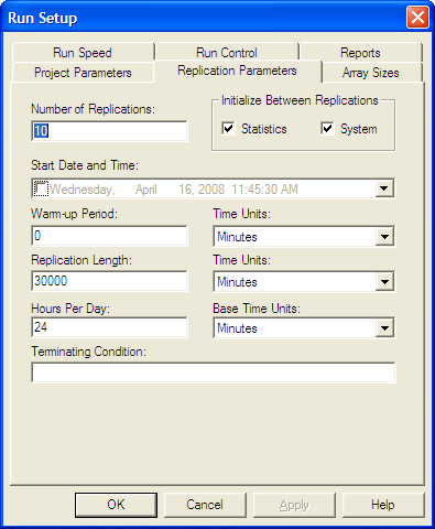
Figure 5.14: Replication parameters for the warm up analysis
The replication length, \(T_e\), is the time when the simulation will end. The Base Time Units can be specified for how the statistics on the default reports will be interpreted and represents the units for TNOW. The Time Units for the Warm-up Period and the Replication Length can also be set. The Warm-up period is the time where the statistics will be cleared. Thus, data will be reported over a net (Replication Length – Warm-up Period) time units.
In order to process the recorded data from the simulation outside of Arena, you must specify that the program produce a text file rather than a dat file. To make this happen we need to indicated to Arena that output files should be written as text using the Run Setup \(>\) Run Control \(>\) Advanced dialog as shown in Figure 5.15. If this option is checked, all statistical data saved to files will be in a CSV format. Since we already ensured that the name of the file had the (.csv) extension this will facilitate Excel recognizing the file as a comma separate variable (CSV) file. Thus, when you double-click on the file, the file will be opened within programs that recognize the CSV format, such as Excel.
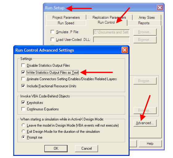
Figure 5.15: Writing statistics output files as text.
Running the simulation will generate two files numInQ.csv and qtime.csv within the current working directory for the model.
Figure 5.16 illustrates the structure of the resulting text file that is produced when using the Write Statistics Output Files as Text option. Each time a new observation is recorded (either time-based or observation based), the time of the observation and the value of the observation is written to the file. When multiple replications are executed, the number (-1) is used in the time field to indicate that a replication has ended. Using these file characteristics, software can be written to post-process the csv files in any fashion that is required for the analysis.
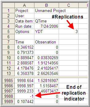
Figure 5.16: Resulting CSV file as shown in Excel.
There is one caveat with respect to using Excel. Excel is limited to 1,048,576 rows of data. If you have \(m\) observations per replication and \(r\) replications then \(m \times r + (r + 7)\) needs to be less than 1,048,576. Thus, you may easily exceed the row limit of Excel by having too many replications and too many observations per replication. Regardless of whether or not the file can be opened in Excel, it still is a valid csv file and can be post processed.
To facilitate the making of Welch plots from Arena output files, I created a program that will read in the Arena text output file and allow the user to make a Welch plot as well as reformat the data to a more convenient CSV structure. The next section will overview the use of that software.
5.3.1 Looking for the Warm up Period in the Welch Plot Analyzer
As previously discussed, the Welch plot is a reasonable approach to assessing the warm up period. Unfortunately, the Arena does not automatically perform a Welch plot analysis. Before proceeding making Welch plots, there is still one more technical challenge related to the post-processing of time-persistent data that must be addressed.
Time-persistent observations are saved within a file from within the model such that the time of the observation and the value of the state variable at the time of change are recorded. Thus, the observations are not equally spaced in time. In order to make a Welch plot, we need to discretize the observations into intervals of time that are equally spaced on the time axis.
Suppose that you divide \(T_e\) into \(k\) intervals of size \(\Delta t\), so that \(T_e = k \times \Delta t\). The time average over the \(j^{th}\) interval is given by:
\[\bar{Y}_{rj} = \dfrac{1}{\Delta t} \int_{j-1) \Delta t}^{j \Delta t} Y_r(t)\mathrm{d}t\]
Thus, the overall time average can be computed from the time average associated with each interval as shown below:
\[\begin{aligned} \bar{Y}_{r} & = \dfrac{\int_0^{T_e} Y_r (t)dt}{T_e} =\dfrac{\int_0^{T_e} Y_r (t)dt}{k \Delta t} \\ & = \dfrac{\sum_{j=1}^{k}\int_{(j-1) \Delta t}^{j \Delta t} Y_r (t)dt}{k \Delta t} = \dfrac{\sum_{j=1}^{k} \bar{Y}_{rj}}{k}\end{aligned}\]
Each of the \(\bar{Y}_{rj}\) are computed over intervals of time that are equally spaced and can be treated as if they are tally based data. Figure 5.17 illustrates the concept of discretizing time-persistent data.
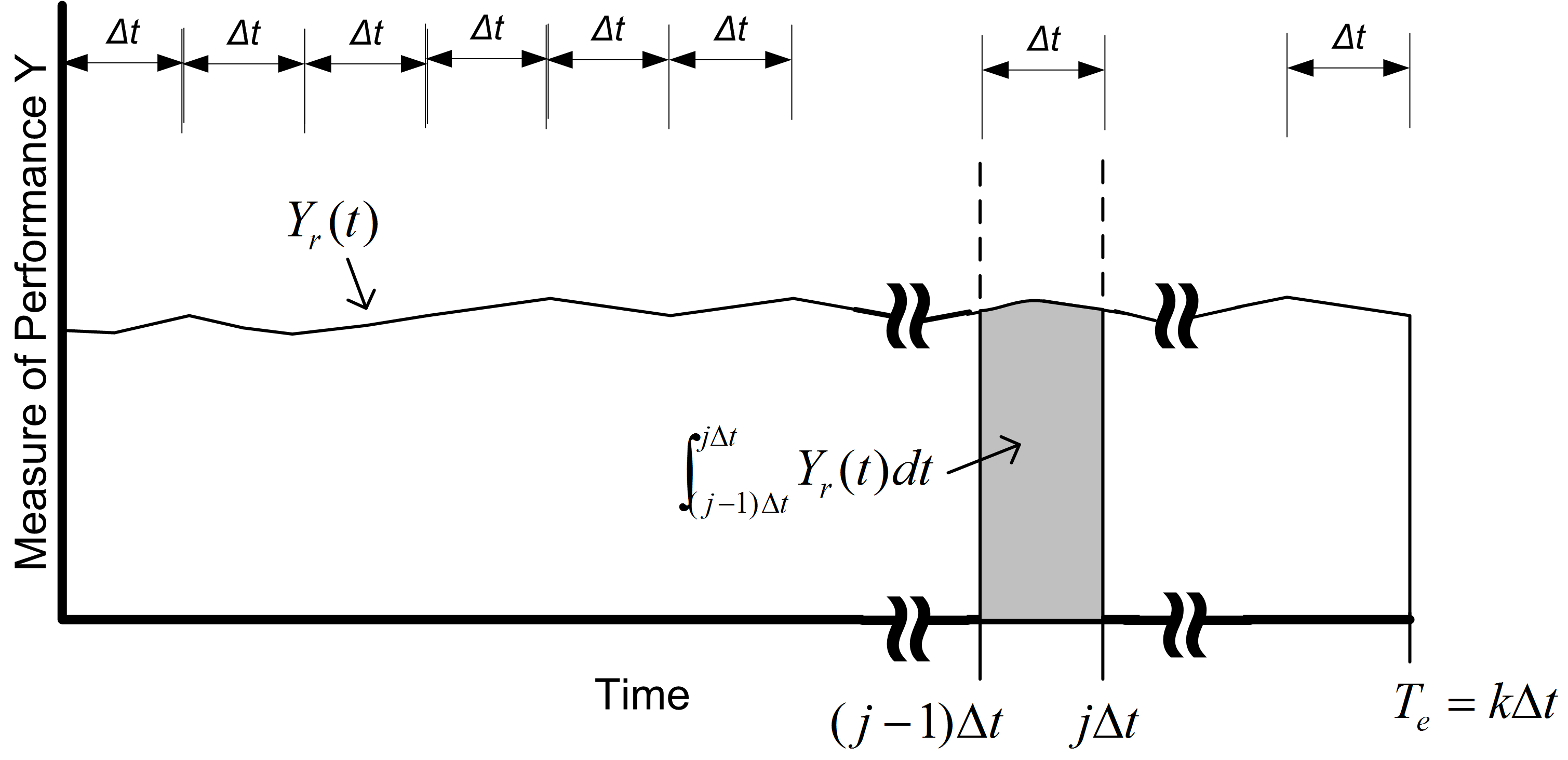
Figure 5.17: Discretizing time persistent observations
The computation of the \(\bar{Y}_{rj}\) for time-persistent data can be achieved when processing the text file written by Arena.
Recall that the data for the Welch analysis is as follows, \(Y_{rj}\) is the \(j^{th}\) observation on replication \(r\) for \(j = 1,2,\cdots,m_r\) where \(m_r\) is the number of observations in the \(r^{th}\) replication, and \(r = 1,2,\cdots,n\). The the Welch averages are computed across the replications for each \(j = 1, 2, \ldots, m\), where \(m = min(m_r)\) for \(r = 1,2,\cdots,n\).
\[ \bar{Y}_{\cdot j} = \dfrac{1}{n}\sum_{r=1}^n Y_{rj} \]
Welch plot data has two components, the Welch averages (\(\bar{Y}_{\cdot j}\) for \(j = 1, 2, \ldots, m\)), and the cumulative average over the observations of the Welch averages:
\[ \overline{\overline{Y}}_{k} = \dfrac{1}{k}\sum_{j=1}^{k} \bar{Y}_{\cdot j} \] for \(k = 1, 2, \ldots, m\)).
The Welch Plot Analyzer is a program that I created to facilitate making Welch plots from Arena data. You may find the Welch Plot Analyzer program files in the book support files. The Welch Plot Analyzer has an option for batching the data before making the Welch plot. Figure 5.18 presents the main dialog for the Welch Plot Analyzer. The user can perform four basic tasks:
- Importing and batching observation or time-persistent data from an Arena generated CSV data file
- Plotting an already processed Welch data file
- Writing Welch plot data to a CSV file. The pairs \((\bar{Y}_{\cdot k},\bar{\bar{Y}}_{k})\) are written to the CSV file for each observation, \(k = 1, 2, \ldots, m\)).
- Writing all Welch data to a CSV file. The CSV file will contain each individual replication as a column, with the Welch average and cumulative average as the last two columns.
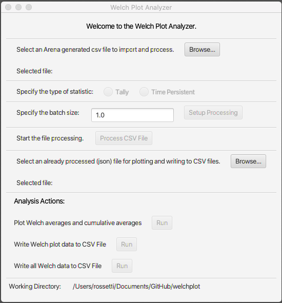
Figure 5.18: Welch Plot Analyzer main dialog
To begin using the Welch Plot Analyzer, use the top most Browse button to select the Arena CSV file that you want to process. After selecting the file, you should specify the type of statistic, either Tally or Time-Persistent. This choice will affect how the batching of the observations is performed.
If the data is tally based, then the batch size is interpreted as the number of observations within each batch. The total number observations, \(m\), is divided into \(k\) batches of size \(b\), where \(b\) is the batch size. It may be useful to batch the observations if \(m\) is very large. However, it is not critical that you specify a batch size other than the default of \(b=1\) for tally based data.
For time-persistent data, the batch size is interpreted as \(\Delta\) as per Figure 5.17. It is useful to specify a \(\Delta\) for discretizing the time-persistent data. The value of \(\Delta\) will default to 1 time unit, which may not be adequate based on the rate of occurrence of the state changes for the time-persistent data. I recommend that \(\Delta\) be set so that about 10 observations on average will fall within each interval. To get an idea for this you can simply open up the Arena generated CSV file and look at the first few rows of the data. By scanning the rows, you can quickly estimate about how much time there needs to be to get about 10 state changes.
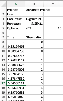
Figure 5.19: Initial rows of number in queue data set.
Reviewing the data for the time-persistent number in queue data as shown in Figure 5.19 indicates that about 10 observations have occurred by time 5. Thus, it seems like having \(\Delta = 5\) would be a reasonable setting.
After setting the batch size, the processing can be set up using the Setup Processing button. This will prepare the data for processing and check if the CSV file is a valid Arena text file. Then, the file can be processed by using the Process CSV File button. Depending on the size of the files, this action may take some time to complete. A dialog will appear when the operation is completed. The processing of the CSV file prepares the data for analysis actions by automatically populating the file for analysis. This file is a JSON file that holds meta-data (data about the data). A second file with a (.wdf) extension is produced that holds the underlying observations in a non-human readable form. The analysis action functionality of the Welch Plot Analyzer allows you to translate the data in the wdf file into a plot or into better organized csv files. Once the file has been processed, the actions within the Analysis Actions section become available. By using the Run button to plot the Welch averages and cumulative averages we produce Figures 5.20 and 5.21. The Welch Plot Analyzer will automatically open up a web browser and display the plots. The plots are based on the plotly open source java script plotting library. In addition, the plots are saved as html to a folder called PlotDir. You can open the html files at any time to review the plots.
Figures 5.20 and 5.21 provide the Welch plots for the time and queue and number in queue data. Notice that the title of the plot contains information that will convert each observation on the x-axis to units of time. For example, on Figure 5.21, we have that each observation is equivalent to 5 time units. That is because we discretized the data with \(\Delta = 5\). Looking at the plot, it appears that the cumulative average converges after observation number 1000. Thus, to set the warm up period, we take \(d=1000\) and \(\Delta=5\) for \(T_w = d \times \Delta = 1000 \times 5 = 5000\). In Figure 5.20, we see that their is a 1 to 1 correspondence between the observation number and time. This is because we get an arrival about every minute. Thus, looking at the plot, it seems that \(d=6000\) is a good deletion point, which translated to \(T_w = 6000\). We will set the warm up period of the simulation to the larger of the two \(T_w\) values (i.e. \(T_w = 6000\))
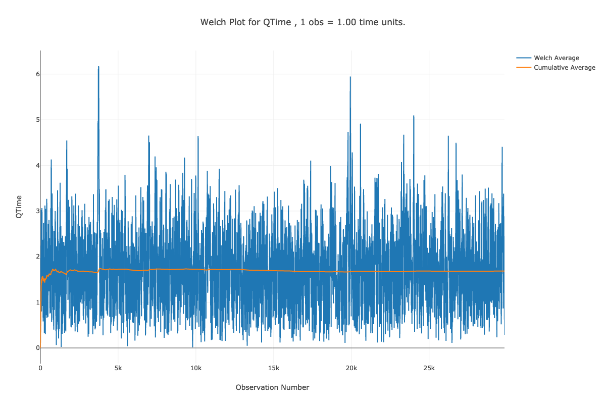
Figure 5.20: Welch plot for time in queue data.
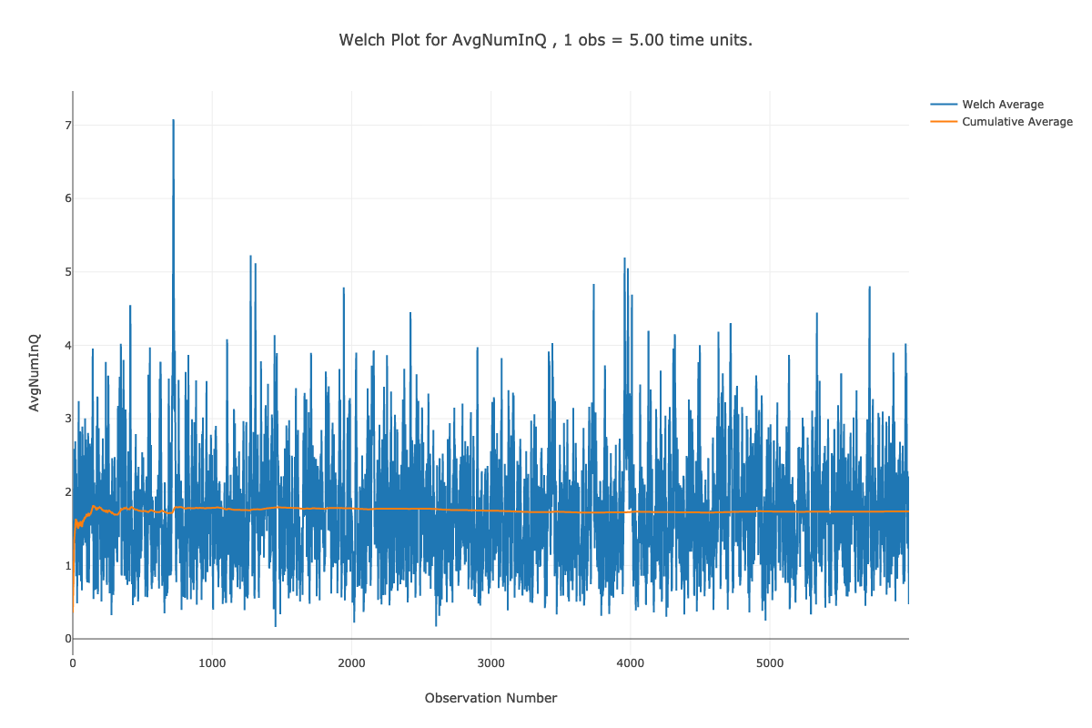
Figure 5.21: Welch plot for number in queue data.
Once you have performed the warm up analysis, you still need to use your simulation model to estimate system performance. Because the process of analyzing the warm up period involves saving the data you could use the already saved data to estimate your system performance after truncating the initial portion of the data from the data sets. If re-running the simulation is relatively inexpensive, then you can simply set the warm up period in the Run Setup \(>\) Replication Parameters dialog and execute the model. Following the rule of thumb that the length of the run should be at least 10 times the warm up period, the simulation was re-run with the settings given in Figure 5.23 (30 replications, 6000 minute warm up period, 60,000 minute replication length). Since the true waiting time in the queue is \(1.6\bar{33}\), it is clear that the 95% confidence interval contains this value. Thus, the results shown in Figure 5.22 indicate that there does not appear to be any significant bias with these replication settings.
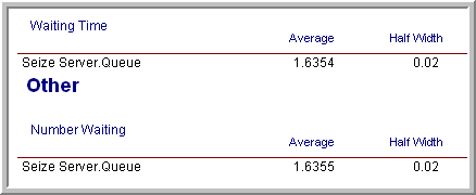
Figure 5.22: Results based on 30 replications.
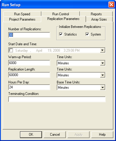
Figure 5.23: Replication-Deletion settings for the example.
The process described here for determining the warm up period for steady state simulation is tedious and time consuming. Research into automating this process is still an active area of investigation. The recent work by (Robinson 2005) and Rossetti and Li (2005) holds some promise in this regard; however, there remains the need to integrate these methods into computer simulation software. Even though determining the warm up period is tedious, some consideration of the warm up period should be done for infinite horizon simulations.
Once the warm up period has been found, you can set the Warm-up Period field in the Run Setup \(>\) Replication Parameters dialog to the time of the warm up. Then, you can use the method of replication-deletion to perform your simulation experiments. Thus, all the discussion previously presented on the analysis of finite horizon simulations can be applied.
When determining the number of replications, you can apply the fixed sample size procedure after performing a pilot run. If the analysis indicates that you need to make more runs to meet your confidence interval half-width you have two alternatives: 1) increase the number of replications or 2) keep the same number of replications but increase the length of each replication. If \(n_0\) was the initial number of replications and \(n\) is the number of replications recommended by the sample size determination procedure, then you can instead set \(T_e\) equal to \((n/n_0)T_e\) and run \(n_0\) replications. Thus, you will still have approximately the same amount of data collected over your replications, but the longer run length may reduce the effect of initialization bias.
As previously mentioned, the method of replication-deletion causes each replication to delete the initial portion of the run. As an alternative, you can make one long run and delete the initial portion only once. When analyzing an infinite horizon simulation based on one long replication, a method is needed to address the correlation present in the within replication data. The method of batch means is often used in this case and has been automated in many simulation packages. The next section discusses the statistical basis for the batch means method and addresses some of the practical issues of using it within Arena.