6.5 Holding and Signaling Entities
In this section we will explore the use of two new modules: HOLD and SIGNAL. The HOLD module allows entities to be held in a queue based on three different options: 1) wait for signal, 2) infinite hold, and 3) scan for condition. The SIGNAL module broadcasts a signal to any HOLD modules that are listening for the specified signal.
To understand the usage of the HOLD module, we must better understand the three possible options:
Wait for Signal – The wait for signal option holds the entities in a queue until a specific numerical value is broadcast via a SIGNAL module. The numerical value is specified via the Wait for Value field of the module. This field can be a constant, an expression (that evaluates to a number), or even an attribute of an entity. In the case of an attribute, each incoming entity can wait for a different numerical value. Thus, when entities waiting for a specific number are signaled with that number, they exit the HOLD module. The other entities stay in the queue.
Infinite Hold – The infinite hold option causes the entities to wait in the queue until they are physically removed (via a REMOVE module).
Scan for Condition – The scan for condition option holds the entities in the queue until a specific condition becomes true within the model. Every time an event occurs within the model, all of the scan for conditions are evaluated. If the condition is true, the waiting entities are permitted to leave the module immediately (at the current time). Since moving entities may cause conditions to change, the check of the condition is performed until no entities can move at the current time. As discussed in Chapter 2, this essentially allows entities to move from the waiting state into the ready state. Then the next event is executed. Because of the condition checking overhead, models that rely on scan for condition logic may execute more slowly.
In the wait for signal option, the entities wait in a single queue, even though the entities may be waiting on different signal values. The entities are held in the queue according to the queue discipline specified in the QUEUE module. In Figure 2.73 of Chapter 2, the entities are in the condition delayed state, waiting on the condition of particular signal. The default discipline of the queue is first in, first out. There can be many different HOLD modules that have entities listening for the same signal within a model. The SIGNAL is broadcast globally and any entities waiting on the signal are released and moved into the ready state. The order of release is essentially arbitrary if there is more than one HOLD module with entities waiting on the signal. If you need a precise ordering of release, then send all entities to another queue that has the desired ordering (and then release them again), or use a HOLD/REMOVE combination instead.
The infinite hold option places the entities in the dormant state discussed in Chapter 2. The entities will remain in the queue of the HOLD module until they are removed by the active entity via a REMOVE or PICKUP module. An example of this is presented in Section 6.6.3.
The scan for condition option is similar in some respects to the wait for signal option. In the scan for condition option, the entities are held in the queue (in the condition delayed state) until a specific condition becomes true. However, rather than another entity being required to signal the waiting entities, the simulation engine notifies waiting entities if the condition become true. This eases the burden on the modeler but causes more computational time during the simulation. In almost all instances, a HOLD with a scan for condition option can be implemented with a HOLD and a wait for signal option by carefully thinking about when the desired condition will change and using an entity to send a signal at that time.
In my opinion, modelers that use the scan for condition option are ill-informed. You can always replace a scan for condition HOLD module with the wait and signal option if you can identify where the condition changes. This is always more efficient. The only time that I would use a the scan for condition option is if there were many (more than 5) locations in the model where the condition could change. Do not fall in love with the scan for condition option. If you know what you are doing, you almost never need to use the scan for condition option and using the scan for condition option almost always indicates that you do not know what you are doing!
6.5.1 Redoing the M/M/1 Model with HOLD/SIGNAL
In this section, we will take the very familiar single server queue and utilize the HOLD/SIGNAL combination to implement it in a more general manner. This modeling will illustrate how the coordination of HOLD and SIGNAL must be carefully constructed. Recall that in a single server queueing situation customers arrive and request service from the server. If the server is busy, the customer must wait in the queue; otherwise, the customer enters service. After completing service the customer then departs.
Assume that we have a single server that performs service according to an exponential distribution with a mean of 0.7 hours. The time between arrival of customers to the server is exponential with mean of 1 hour. If the server is busy, the customer waits in the queue until the server is available. The queue is processed according to a first in, first out rule.
6.5.1.1 First Solution to M/M/1 with HOLD/SIGNAL Example
In this solution, we will not use a RESOURCE module. Instead, we will use
a variable, vServer, that will represent whether or not the server is
busy. When the customer arrives, we will check if the server is busy. If
so, the customer will wait until signaled that the server is available.
The pseudo-code for this example is given in the following pseudo-code.
CREATE customer every EXPO(1)
ASSIGN myArriveTime = TNOW
DECIDE
    IF vServer == 1
        BEGIN HOLD Server Queue
            Wait for End Service Signal
      END HOLD
    ENDIF
END DECIDE
ASSIGN vServer = 1
DELAY for EXPO(0.7)
ASSIGN vServer = 0
DECIDE
    IF Server Queue is not empty
        BEGIN SIGNAL End Service
            Signal Limit = 1
        END SIGNAL
    ENDIF
END DECIDE
RECORD TNOW - myArriveTime
DISPOSE
The customer is created and then the time of
arrival is recorded in the attribute myArriveTime. If the server is
busy, vServer == 1, then the customer goes into the HOLD queue to wait
for an end of service signal. If the server is not busy, the customer,
makes the server busy and then delays for the service time. After the
service is complete, the server is indicated as idle (vServer = 0).
Then, the queue is checked. If there are any customers waiting, a signal
is sent to the HOLD queue to release one customer. Finally, the system
time is recorded before the customer departs the system.
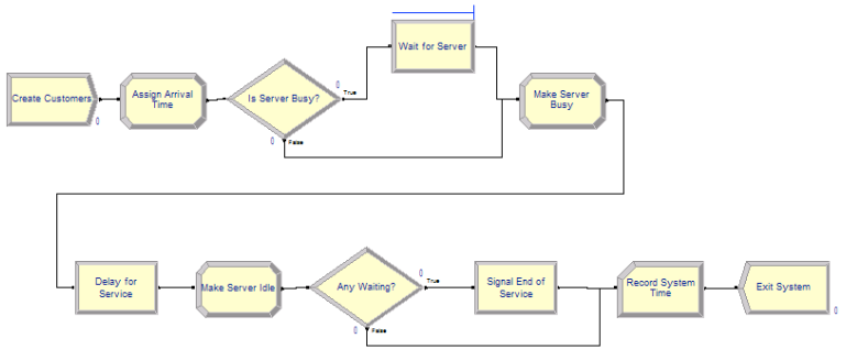
Figure 6.47: First implementation of M/M/1 system with HOLD and SIGNAL
Figure 6.47 illustrates the flow chart for the implementation. The model represents the pseudo-code almost verbatim. The new HOLD and SIGNAL modules are shown in Figure 6.48 and Figure 6.49, respectively. The completed model can be found in file FirstMM1HoldSignal.doe found in the chapter files.
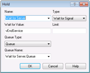
Figure 6.48: HOLD module for first M/M/1 implemenation
Notice that the HOLD module has an option drop down menu that allows the user to select one
of the aforementioned hold options. In addition, the Wait For Value
field indicates the value on which the entities will wait. Here is it a
variable called vEndService. It can be any valid expression that
evaluates to an integer. The Limit field (blank in this example) can be
used to set to limit how many entities will be released when the signal
is received.
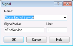
Figure 6.49: SIGNAL module for first M/M/1 implemenation
Figure 6.49 shows the SIGNAL module. The Signal Value field indicates the signal that will be broadcast. The Limit field indicates the number of entities to be released when the signal is completed. In this case, because the server works on 1 customer at at time, the limit value is set to 1. This causes 1 customer to be released from the HOLD, whenever the signal is sent.
Figure 6.50 presents the result from running the model for 30 replications with warm up of 30,000 hours and a run length of 80,000. The results match very closely the theoretical results for this M/M/1 situation.
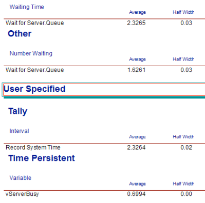
Figure 6.50: Results for first M/M/1 implemenation
There is one key point to understand in this implementation. What would happen if we did not first check if the server was busy before going into the HOLD queue? If we did not do this, then no customers would ever get signaled! This is because, the signal comes at the end of service and no customers would ever reach the SIGNAL (because they would all be waiting for the signal that is never coming). This is a common modeling error when first using the HOLD/SIGNAL combination.
A fundamental aspect of the HOLD/SIGNAL modeling constructs is that entities waiting in the HOLD module are signaled from a SIGNAL module. In the last example, the departing entity signaled the waiting entity to proceed. In the next implementation, we are going to have two types of entities. One entity will represent the customer. The second entity will represent the server. We will use the HOLD/SIGNAL constructs to communicate between the two processes.
6.5.1.2 Second Solution to M/M/1 with HOLD/SIGNAL Example
In this implementation, we will have two process flows, one for the customers and one for the server. At first, this will seem very strange. However, this approach will enable a great deal of modeling flexibility. Especially important is the notion of modeling a resource, such as a server, with its own process. Modeling a resource as an active component of the system (rather than just passively being called) provides great flexibility. Flexibility that will serve you well when approaching some complicated modeling situations. The key to using to two process flows for this modeling is to communicate between the two processes via the use of signals.
Figure 6.51 presents the model for this second implementation. Note the two process flows in the figure. The file SecondMM1HoldSignal.doe contains the details.
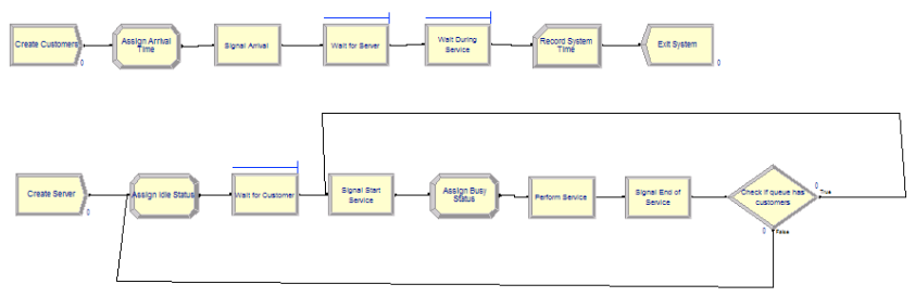
Figure 6.51: Second implementation of the M/M/1 with HOLD and SIGNAL
The logic follow very closely the pseudo-code provided in the following pseudo-code.
CREATE customer every EXPO(1)
ASSIGN myArriveTime = TNOW
SIGNAL server of arrival
    Signal Value = vArrivalSignal
END SIGNAL
HOLD in Server Queue
    Wait for Begin Service Signal
END HOLD
HOLD in Service Queue
    Wait for End Service Signal
END HOLD
RECORD TNOW - myArriveTime
DISPOSE of customer

CREATE 1 server at time 0.0
LABEL: A
ASSIGN vServerStatus = 0
HOLD Wait for Customer arrival signal
  Wait for Value = vArrivalSignal
END HOLD
LABEL: B
SIGNAL Start Service
    Signal Value = vStartService
    Signal Limit = 1
END SIGNAL
ASSIGN vServerStatus = 1
DELAY for EXPO(0.7)
SIGNAL End Service
    Signal Value = vEndService
    Signal Limit = 1
END SIGNAL
DECIDE
    IF Server Queue is not empty
        GOTO to LABEL B:
    ELSE
        GOTO to LABEL A:
    ENDIF
END DECIDE
In the pseudo-code, the first CREATE module creates customers according to the exponential time between arrivals and then the time of arrival is noted in order to later record the system time. Next, the customer signals that there has been an arrival. Think of it as the customer ringing the customer service bell at the counter. The customer then goes into the HOLD to await the beginning of service. If the server was busy when the signal went off, the customer just continues to wait. If the server was idle (waiting for a customer to arrive), then the server moves forward in their process to signal the customer to start service. When the customer gets the start service signal, the customer moves immediately into another HOLD queue. This second hold queue provides a place for the customer to wait while the server is performing the service. When the end of service signal occurs the customer departs after recording the system time.
The second CREATE module, creates a single entity that represents the server. Essentially, the server will cycle through being idle and busy. After being created the server sets its status to idle (0) and then goes into a HOLD queue to await the first customer’s arrival. When the customer arrives, the customer sends a signal. The server can then proceed with service. First, the server signals the customer that service is beginning. This allows the customer to proceed to the hold queue for service. Then, the server delays for the service time. After the service time is complete, the server signals the customer that the end of service has occurred. This allows the customer to depart the system. After signaling the end of service, the server checks if there are any waiting customers, if there are waiting customers, the entity representing the server is sent to Label B to signal a start of service. If there are no customers waiting, then the entity representing the server is sent to Label A, to wait in a hold queue for the next customer to arrive.
This signaling back and forth must seem overly complicated. However, this example illustrates how two entities can communicate with signals. In addition, the notion of modeling a server as a process should open up some exciting possibilities. The modeling of a server as a process permits very complicated resource allocation rules to be embedded in a model.
Consider modeling resources as entities. This allows logic to be used to model how the resource behaves given the state of the system. This is an excellent way to model resources as intelligent agents.
6.5.2 Using Wait and Signal to Release Entities
In many situations, entities will need to wait until a specific time or condition occurs within a system. One classic example of this is order picking waves within a distribution facility. In this situation, orders (the entities) will arrive throughout the day and be held until a particular time that they can be released. The release of sets of the orders is timed to correspond to particular periods of time. In the parlance of distribution center picking operations, these periods are called waves, like waves hitting a beach.
The length and timing of the waves is typically determined by some optimization algorithm that ensures that the picking operations can be completed in an optimal manner in time for the subsequent shipping of the items. In addition, each order is assigned (again according to some optimization method) to a particular period (wave). For simplicity, we will assume that the periods (waves) are one hour long and that the orders are randomly assigned to each wave. Again, these assignments are often much more complex.
In this section, we will examine how to release picking orders within a distribution center under the following assumptions:
Assume that at the beginning of a shift there are a number of orders that need to be picked within the warehouse
Let N be the number of orders to pick
Assume that N ~ Poisson (mean rate = 100 orders/day)
Assume that the warehouse has 4 picking periods (1, 2, 3, 4)
The first picking period starts at time 0.0
Each picking period lasts 60 minutes
Assume that the orders are equally likely to be assigned to any of the four periods
After the orders are released, they proceed to pickers who pick the orders and send them to be shipped.
- Assume that the time to pick the entire order is TRIA(5, 10, 15) minutes
Build and Arena model to simulate this system over the picking periods
- Determine the number of pickers needed to satisfactorily complete the picking operations.
The purpose of this example is to illustrate the basic ideas of using the wait and signal functionality of Arena to release the orders. The basic strategy will be to assign to each order a number that indicates when it should be released. In other words, we assign its release period (or wave). Then, the arriving order will wait in a HOLD module for the appropriate signal representing the start of its period. At which time, the order will be released to pickers for processing.
The first modeling issue is to represent is the creation of the orders. In a typical distribution center setting the customer orders may arrive throughout the day; however, they are typically not processed immediately upon arrival. In most situations, they are processed by the order processing systems of the distribution center (human or computer) and made ready for release. There is typically a random number of orders to be processed. For simplicity in this example, we will assume that the number of orders per day is well modeled with a Poisson distribution with a mean rate of 100 per day. Thus, at the beginning of the day all orders are available and assigned their release period. Let’s assume that there will be four release periods, each spaced 1 hour apart with the first period starting at time 0.0 and lasting one hour. Thus, the second period starts at time 1.0, and lasts an hour, etc. We will number the (waves) periods 1, 2, 3, 4.
Because of our assumption that orders are randomly assigned to waves, we need a distribution to represent this assignment. To keep it simple, we will assume that the orders are equally likely to be assigned any of the periods 1, 2, 3, 4. Thus, we need to generate a discrete uniform random variate over the range from 1 to 4. Recall that the Arena formula for generating a DU(a,b) random variate, X, is:
X = a + AINT((b - a + 1)*UNIF(0,1))
Thus, to generate DU(1,4), we have,
1 + AINT((4 - 1 + 1)*UNIF(0,1)) = 1 + AINT(4*UNIF(0,1))
Again, in general, the assignment of orders to particular picking periods (waves) is often a much more complex process that takes into account the order due dates, the work associated with the orders, and the locations of the items to be picked.
Let’s take a look at the pseudo-code to create and hold the orders for later release.
ATTRIBUTES: myWave // to hold which picking wave to listen for
--
CREATE POIS(100) entities with 1 event at time 0.0
ASSIGN myWave = 1 + AINT(4*UNIF(0,1))
HOLD wait for signal myWave
Go To: Label Picking Process
That’s it! This will create the orders, assign their wave number and cause them to wait within a HOLD module for a signal that is specified by the value of the attribute, myWave. When this signal (number) is broadcast by a SIGNAL module all the entities (orders) waiting in the HOLD queue for that corresponding wave number will be released and proceed for further processing.
The second modeling issue is to represent the timing and signaling of the picking waves. To implement this situation, we will create a “clock-entity” that determines the period and makes the signal. For this situation we will use a global variable, vPeriod, that keeps track of the current period and is used to signal the start of the period.
Now, we have one tricky issue to address. The start of the first wave happens at time 0.0, but as noted in the previous pseudo-code, the orders for the day are also created at time 0.0. We need to coordinate between two CREATE modules to ensure that the clock-entity allows the orders to be created first. We must ensure that the orders are in the HOLD module before the signal for the first wave occurs; otherwise, the orders associated with the first wave will not be in the HOLD queue when the signal occurs. Thus, they will miss the first signal and not be released.
While there are number of ways to address this issue, the simplest is to cause the clock-entity to be created infinitesimally after time 0.0. This will allow all the entities (orders) from the order creation process to be created and go into the HOLD module queue before the clock-entity signals the start of the first wave. Let’s take a look at the pseudo-code for this situation.
We will use three variables to represent the time periods.
VARIABLES:
vPeriod = 0 // to track the current period
vPeriodLength = 60 // minutes per period
vLastPeriod = 4 // the number of periods
Then, we will use a logical entity, call it the clock-entity, that will loop around signaling the appropriate period. In essence, it is ticking off the periods through time. This is a very common modeling pattern.
CREATE 1 entity at time 0.0001
A:
ASSIGN vPeriod = vPeriod + 1
If vPeriod \> vLastPeriod
DISPOSE
ELSE
SIGNAL vPeriod
DELAY vPeriodLength minutes
Go to: Label A
Notice that in this pseudo-code there are two defined variables
(vPeriodLength and vLastPeriod) to make the code more generic. Using
these variables, we can easily vary the number of periods and the length
of each period. Notice also that the CREATE module indicates that the
clock entity is created at time 0.0001. This ensures that the CREATE
module associated with creating the orders goes first (at time 0.0) and
allows the orders to fill up the HOLD queue. The clock-entity then
increments the variable, vPeriod, so that the current period (wave) is
noted. We then check if the current period is greater than the last
period to simulate. If so, the clock-entity is disposed.
If the last period has not happened, we need to signal the start of the
period. When the clock-entity executes the SIGNAL module, the value of
the signal (vPeriod) is broadcast globally throughout the model. Any
entities in any HOLD modules that are waiting for that particular
number as their signal will be removed from the HOLD queue and placed in
the ready state to be processed at the current time. Since the
clock-entity immediately enters a DELAY module, it is placed in the
time-delayed state to become the active entity 60 minutes later. Thus,
all the entities that were signaled can now be processed. According to
our previous pseudo-code, they will go to the label Picking Process.
As noted previously, there are a number of other ways to coordinate the timing of the order process and the wave process to ensure that the orders are placed in the HOLD queue before the clock-entity makes the first signal. Rather than using an infinitesimal delay as illustrated here, you could remove the CREATE module for the clock-entity. To ensure that the clock-entity is made after the orders are made, you can have the order making process create the clock-entity. One way to do this is to have the first order created go through a SEPARATE module. The duplicate entity will be the clock entity and it would be sent to the logic that signals the waves (pseudo code labeled A). Because a SEPARATE module places the duplicate entities in the ready state, the clock-entity will not proceed until the orders are all waiting. The interested reader is encouraged to test their knowledge by implementing this approach. The implementation and analysis of this example within Arena is left as an exercise.
In the next section, we see how essential the wait and signal constructs are to the modeling of an important situation within inventory systems.
6.5.3 Modeling a Reorder Point, Reorder Quantity Inventory Policy
In an inventory system, there are units of an item (e.g. computer printers, etc.) for which customers make demands. If the item is available (in stock) then the customer can receive the item and depart. If the item is not on hand when a demand from a customer arrives then the customer may depart without the item (i.e. lost sales) or the customer may be placed on a list for when the item becomes available (i.e. back ordered). In a sense, the item is like a resource that is consumed by the customer. Unlike the previous notions of a resource, inventory can be replenished. The proper control of the replenishment process is the key to providing adequate customer service. There are two basic questions that must be addressed when controlling the inventory replenishment process: 1) When to order? and 2) How much to order?. If the system does not order enough or does not order at the right time, the system not be able to fill customer demand in a timely manner. Figure 6.52 illustrates a simple inventory system.
Figure 6.52: A simple reorder point, reorder quantity inventory system
There are a number of different ways to manage the replenishment process for an inventory item. These different methods are called inventory control policies. An inventory control policy must determine (at the very least) when to place a replenishment order and how much to order. This section examines the use of a reorder point (\(r\)), reorder quantity (\(Q\)) inventory policy. This is often denoted as an \((r, Q)\) inventory policy. The modeling of a number of other inventory control policies will be explored as exercises. After developing a basic understanding of how to model an \((r, Q)\) inventory system, the modeling can be expanded to study supply chains. A supply chain can be thought of as a network of locations that hold inventory in order to satisfy end customer demand.
The topic of inventory systems has been well studied. A full exposition of the topic of inventory systems is beyond the scope of this text, but the reader can consult a number of texts within the area, such as (Hadley and Whitin 1963), (Axsäter 2006), Silver, Pyke, and Peterson (1998), or (Zipkin 2000) for more details. The reader interested in supply chain modeling might consult (Nahmias 2001), (Askin and Goldberg 2002), (Chopra and Meindl 2007), or (Ballou 2004).
Within this section we will develop a model of a continuous review \((r, Q)\) inventory system with back-ordering. In a continuous review \((r, Q)\) inventory control system, demand arrives according to some stochastic process. When a demand (customer order) occurs, the amount of the demand is determined, and then the system checks for the availability of stock. If the stock on-hand is enough for the order, the demand is filled and the quantity on-hand is decreased. On the other hand, if the stock on-hand is not enough to fill the order, the entire order is back-ordered. The back-orders are accumulated in a queue and they will be filled after the arrival of a replenishment order. Assume for simplicity that the back-orders are filled on a first come first served basis. The inventory position (inventory on-hand plus on-order minus back-orders) is checked each time after a regular customer demand and the occurrence of a back-order. If the inventory position reaches or falls under the reorder point, a replenishment order is placed. The replenishment order will take a possibly random amount of time to arrive and fill any back-orders and increase the on-hand inventory. The time from when a replenishment order is placed until the time that it arrives to fill any back-orders is often called the lead time for the item.
There are three key state variables that are required to model this situation. Let \(I(t)\), \(\mathit{IO}(t)\), and \(\mathit{BO}(t)\) be the amount of inventory on hand, on order, and back-ordered, respectively at time \(t\). The net inventory, \(\mathit{IN}(t) = I(t) - \mathit{BO}(t)\), represents the amount of inventory (positive or negative). Notice that if \(I(t) > 0\), then \(\mathit{BO}(t) = 0\), and that if \(\mathit{BO}(t) > 0\), then \(I(t) = 0\). These variables compose the inventory position, which is defined as:
\[\mathit{IP}(t) = I(t) + \mathit{IO}(t) - \mathit{BO}(t)\]
The inventory position represents both the current amount on hand, \(I(t)\), the amounted back ordered, \(\mathit{BO}(t)\), and the amount previously ordered, \(\mathit{IO}(t)\). Thus, when placing an order, the inventory position can be used to determine whether or not a replenishment order needs to be placed. Since, \(\mathit{IO}(t)\), is included in \(\mathit{IP}(t)\), the system will only order, when outstanding orders are not enough to get \(\mathit{IP}(t)\) above the reorder point.
In the continuous review \((r, Q)\) policy, the inventory position must be checked against the reorder point as demands arrive to be filled. After filling (or back-ordering) a demand, either \(I(t)\) or \(\mathit{BO}(t)\) will have changed (and thus \(\mathit{IP}(t)\) will change). If \(\mathit{IP}(t)\) changes, it must be checked against the reorder point. If \(\mathit{IP}(t) \leq r\), then an order for the amount \(Q\) is placed.
For simplicity, assume that each demand that arrives is for 1 unit. This simplifies how the order is processed and the processing of any back orders. The pseudo-code for this situation is given the following pseudo-code.
CREATE demand
ASSIGN myAmtDemanded = 1
Send to LABEL: Order Fulfillment

LABEL: Order Fulfillment
DECIDE
    IF I(t) >= myAmtDemanded THEN //fill the demand
        ASSIGN I(t) = I(t) - myAmtDemanded
    ELSE // handle the backorder
        ASSIGN BO(t) = BO(t) + myAmtDemanded
        SEPARATE Duplicate 1 entiy
            Send duplicate to LABEL: Handle Back Order
    ENDIF
  ASSIGN IP(t) = I(t) + IO(t) - BO(t)$
  Send to LABEL: Replenishment Ordering
END DECIDE

LABEL: Handle Back Order
HOLD Back order queue: wait for signal
    On Signal: release all from queue
END HOLD
ASSIGN BO(t) = BO(t) - myAmtDemanded
Send to LABEL: Order Fulfillment

LABEL: Replenishment Ordering
IF IP(t) <= r
    ASSIGN IO(t) = IO(t) + Q //place the order
    DELAY for lead time
    ASSIGN IO(t) = IO(t) - Q //receive the order
    ASSIGN I(t) = I(t) + Q
    SIGNAL: Hold back order queue
ENDIF
DISPOSE
Referring to the pseudo-code, the entity being created is a customer demand.
The amount of the demand should be an attribute (myAmtDemanded) of the
entity having value 1. After the customer arrives, the customer is sent
to order fulfillment. Notice the use of a label to indicate the order
filling logic.
At order fulfillment, we need to check if there is inventory available to satisfy the demand. If the amount required can be satisfied \(I(t) \geq \mathit{myAmtDemanded}\). Then, the on hand inventory is decremented by the amount of the demand. If the demand cannot be satisfied \(I(t) < \mathit{myAmtDemanded}\)). In this case, the amount waiting in the back order queue, \(\mathit{BO}(t)\), is incremented by the amount demanded. Then, a duplicate is made so that the duplicate can be sent to the back order queue.
In either case of filling the demand or not filling the demand, the inventory position must be updated. This is because either \(I(t)\) or \(\mathit{BO}(t)\) changed. Since the inventory position changed, we must check if a replenishment order is necessary. The entity is sent to the replenishment logic.
At the replenishment logic, the inventory position is checked against the reorder point. If the inventory position is less than or equal to the reorder point, an order is placed. If no order is placed, the entity skips over the order placement logic and is disposed. If an order is placed, the on order variable is incremented by the reorder quantity and the delay for the lead time started. Once the lead time activity is completed, the on order and on hand variables are updated and a signal is sent to the back-order queue. A signal is sent to the back order queue so that if there are any demands waiting in the back order queue, the demands can try to be filled.
The key performance measures for this type of system are the average amount of inventory on hand, the average amount of inventory back-ordered, the percentage of time that the system is out of stock, and the average number of orders made per unit time.
Let’s discuss these performance measures before indicating how to collect them within a simulation. The average inventory on hand and the average amount of inventory back-ordered can be defined as follows:
\[\begin{aligned} \bar{I} & = \frac{1}{T}\int_0^T I(t)\mathrm{d}t \\ \overline{\mathit{BO}} & = \frac{1}{T}\int_0^T \mathit{BO}(t)\mathrm{d}t\end{aligned}\]
As can be seen from the definitions, both \(I(t)\) and \(\mathit{BO}(t)\) are time-persistent variables and their averages are time averages. Under certain conditions as \(T\) goes to infinity, these time averages will converge to the steady state performance for the \((r, Q)\) inventory model. The percentage of time that the system is out of stock can be defined based on \(I(t)\) as follows:
\[SO(t) = \begin{cases} 1 & I(t) = 0\\ 0 & I(t) > 0 \end{cases}\]
\[\overline{\mathit{SO}} = \frac{1}{T}\int_0^T \mathit{SO}(t)\mathrm{d}t\]
Thus, the variable \(SO(t)\) indicates whether or not there is no stock on hand at any time. A time average value for this variable can also be defined and interpreted as the percentage of time that the system is out of stock. One minus \(\overline{\mathit{SO}}\) can be interpreted as the proportion of time that the system has stock on hand. Under certain conditions (but not always), this can also be interpreted as the fill rate of the system (i.e. the fraction of demands that can be filled immediately). Let \(Y_i\) be an indicator variable that indicates 1 if the \(i^{th}\) demand is immediately filled (without back ordering) and 0 if the \(i^{th}\) demand is back ordered upon arrival. Then, the fill rate is defined as follows.
\[\overline{\mathit{FR}} = \frac{1}{n} \sum_{i=1}^{n} Y_i\]
Thus, the fill rate is just the average number of demands that are directly satisfied from on hand inventory. The variables \(\overline{\mathit{SO}}\) and \(\overline{\mathit{FR}}\) are measures of customer service.
To understand the cost of operating the inventory policy, the average number of replenishment orders made per unit time or the average order frequency needs to be measured. Let \(N(t)\) be the number of replenishment orders placed in \((0,t]\), then the average order frequency over the period \((0,t]\) can be defined as:
\[\overline{\mathit{OF}} = \frac{N(T)}{T}\]
Notice that the average order frequency is a rate (units/time).
In order to determine the best settings of the reorder point and reorder quantity, we need an objective function that trades-off the key performance measures within the system. This can be achieved by developing a total cost equation on a per time period basis. Let \(h\) be the holding cost for the item in terms of $/unit/time. That is, for every unit of inventory held, we accrue \(h\) dollars per time period. Let \(b\) be the back order cost for the item in terms of $/unit/time. That is, for every unit of inventory back ordered, we accrue \(b\) dollars per time period. finally, let \(k\) represent the cost in dollars per order whenever an order is placed. The settings of the reorder point and reorder quantity depend on these cost factors. For example, if the cost per order is very high, then we should not want to order very often. However, this means that we would need to carry a lot of inventory to prevent a high chance of stocking out. If we carry more inventory, then the inventory holding cost is high.
The average total cost per time period can be formulated as follows:
\[\overline{\mathit{TC}} = k\overline{\mathit{OF}} + h\bar{I} + b\overline{\mathit{BO}}\]
A discussion of the technical issues and analytical results related to these variables can be found in Chapter 6 of (Zipkin 2000). Let’s take a look at an example that illustrates an inventory situation.
Average inventory on hand and back ordered
Average frequency at which orders are placed
Probability that an arriving customer does not have their demand immediately filled
Average total cost per time
The Arena model will follow closely the previously discussed pseudo-code. To develop this model, first define the variables to be used as per Figure 6.53. The reorder point and reorder quantity have been set to (\(r = 1\)) and (\(Q = 2\)), respectively. The costs have be set based on the example. Notice that the report statistics check boxes have been checked for the on hand inventory and the back-ordered inventory. This will cause time-based statistics to be collected on these variables.
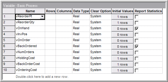
Figure 6.53: Defining the inventory model variables
Figure 6.54 illustrates the logic for creating incoming demands and for order fulfillment. First, an entity is created to represent the demand. This occurs according to a time between arrivals with an exponential distribution with a mean of (1.0/0.12) days (3.6 units/month * (1 month/30 days) = 0.12 units/day).
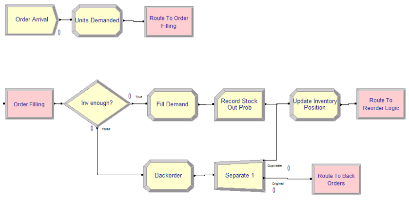
Figure 6.54: Initial order filling logic for the (r, Q) inventory model
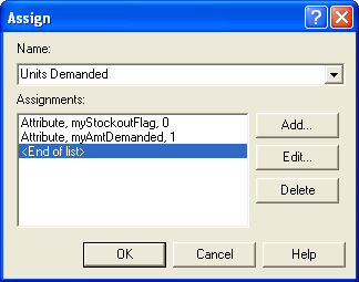
Figure 6.55: Assigning the amount of demand
The ASSIGN module in Figure 6.55 shows the amount demanded set to 1 and a stock out indicator set to zero. This will be used to tally the probability that an incoming demand is not filled immediately from on hand inventory. This is called the probability of stocking out. This is the complement of the fill rate. Then, a ROUTE module with zero transfer delay is used to send the demand to a station to handle the order fulfillment. Note that a STATION was used here to represent a logical label to which an entity can be sent.
At the order fulfillment station, the DECIDE module is used to check if the amount demanded is less than or equal to the inventory on hand. If true, the demand is filled using the ASSIGN module to decrement the inventory on hand. The RECORD module is used to collect statistics for the probability of stock out. The inventory position is updated and then the demand is sent to the reordering logic. If false, the demand is back-ordered. The ASSIGN module labeled Backorder increments the number of back orders. Then the SEPARATE module creates a duplicate, which goes to the station than handles back orders. The original is sent to update the inventory position before being sent to the reordering logic via a ROUTE module.
The Fill Demand, BackOrder, and Update Inventory Position ASSIGN modules have the form shown in Figure 6.56. The amount on hand or the amount back-ordered is decreased or increased accordingly. In addition, the inventory position is updated. In the back-ordering ASSIGN module, the stock out flag is set to 1 to indicate that this particular demand did not get an immediate fill.
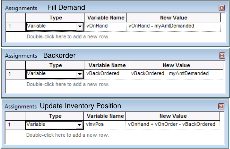
Figure 6.56: ASSIGN modules for filling, backordering, and updating inventory position
When the demand is ultimately filled, it will pass through the RECORD module within Figure 6.54. Notice, that in the RECORD module, the expression option is used to record on the attribute, which has a value of 1 if the demand had been back-ordered upon arrival and the value 0 if it had not been back-ordered upon initial arrival. This indicator variable will estimate the probability that an arriving customer will be back-ordered. In inventory analysis parlance, this is called the probability of stock out. One minus the probability of stock out is called the fill rate for the inventory system. Under Poisson arrivals, it can be shown that the probability of an arriving customer being back-ordered will be the same as \(\overline{\mathit{SO}}\), the percentage of time that the system is stocked out. This is due to a phenomenon called PASTA (Poisson Arrivals See Time Averages) and is discussed in (Zipkin 2000) as well as many texts on stochastic processes (e.g. (Tijms 2003))
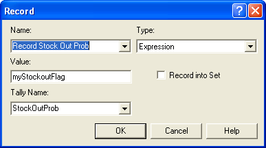
Figure 6.57: Recording the initial fill indicator variable
The logic representing the back ordering and replenishment ordering process is given in Figure 6.58. Notice how STATION modules have been used to denote the start of the logic. In the case of back ordering, the Handle Back Order station has a HOLD module, which will hold the demands waiting to be filled in a queue. See Figure 6.59. When the HOLD module is signaled (value = 1), the waiting demands are released. The release will be triggered after a replenishment order arrives. The number of waiting back orders is decremented in the ASSIGN module and the demands are sent via a ROUTE module for order fulfillment.
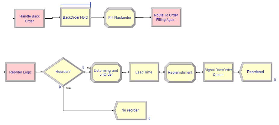
Figure 6.58: Back ordering and replenishment logic
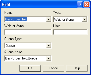
Figure 6.59: Backorder queue as a HOLD module
At the Reorder Logic station, the DECIDE module checks if the inventory position is equal to or below the reorder point. If this is true, then the amount on order is updated. After the amount of the order is determined, the order entity experiences the delay representing the lead time. After the lead time, the order has essentially arrived to replenish the inventory. The corresponding ordering and replenishment ASSIGN modules and the subsequent SIGNAL modules are given in Figure 6.60 and Figure 6.61, respectively.
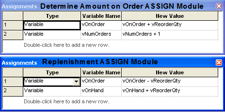
Figure 6.60: Ordering and replenishment ASSIGN modules
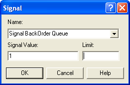
Figure 6.61: Signalling the backorder queue
The basic model structure is now completed; however, there are a few
issues related to the collection of the performance measures that must
be discussed. The average order frequency must be collected. Recall
\(\bar{OF} = N(T)/T\) that . Thus, the number of orders placed within the
time interval of interest must be observed. This can be done by creating
a logic entity that will observe the number of orders that have been
placed since the start of the observation period. In
Figure 6.54, there is a variable called,
vNumOrders, which is incremented each time an order is placed. This
is, in essence, \(N(T)\).
Figure 6.62 shows the order frequency collection
logic. First an entity is created every, \(T\), time units. In this case,
the interval is monthly (every 30 days).
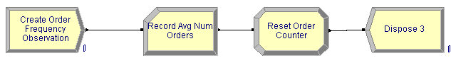
Figure 6.62: Order frequency collection logic
Then the RECORD module, shown in Figure 6.63, observes the value of vNumOrders. The following
ASSIGN module sets vNumOrders equal to zero. Thus, vNumOrders
represents the number of orders accumulated during the 30 day period.
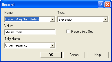
Figure 6.63: Recording the number of orders placed
To close out the statistical collection of the performance measures, the
collection of \(\overline{\mathit{SO}}\) as well as the cost of the policy
needs to be discussed. To collect \(\overline{\mathit{SO}}\), a
time-persistent statistic needs to be defined using the Statistic module
of the Advanced Process panel as in
Figure 6.64. The expression (vOnHand == 0) is
a boolean expression, which evaluates to 1.0 if true and 0.0 if false.
By creating a time-persistent statistic on this expression, the
proportion of time that the on-hand is equal to 0.0 can be tabulated.
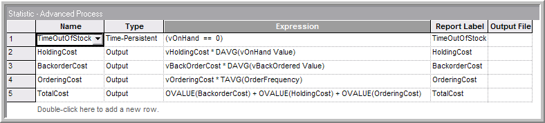
Figure 6.64: Statistic module for (r, Q) inventory model
To record the costs associated with the policy, three Output statistics
are needed. Recall that these are designed to be observed at the end of
each replication. For the inventory holding cost, the time-average of
the on-hand inventory variable, DAVG(vOnHand Value), should be
multiplied by the holding cost per unit per time. The back-ordering cost
is done in a similar manner. The ordering cost is computed by taking the
cost per order times the average order frequency. Recall that this was
captured via a RECORD module every month. The average from the RECORD
module is available through the TAVG() function. Finally, the total
cost is tabulated as the sum of the back-ordering cost, the holding
cost, and the ordering cost. In
Figure 6.64, this was accomplished by using the
OVALUE() function for OUTPUT statistics. This function returns the
last observed value of the OUTPUT statistic. In this case, it will
return the value observed at the end of the replication. Each of these
statistics will be shown on the reports as user-defined statistics. The completed model is found in file rQInventoryModel.doe in the chapter files.
The case of (r = 1, Q = 2) was run for 30 replications with a warm up period of 3600 days and a run length of 39,600 days. Figure 6.65 indicates that the total cost is about 1.03 per month with a probability of stocking out close to 40%. Notice that the stock out probability is essentially the same as the percentage of time the system was out of stock. This is an indication that the PASTA property of Poisson arrivals is working according to theory.
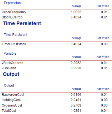
Figure 6.65: Results for the (r, Q) inventory model
This example should give you a solid basis for developing more sophisticated inventory models. While analytical results are available for this example, small changes in the assumptions necessitate the need for simulation. For example, what if the lead times are stochastic or the demand is not in units of 1. In the latter case, the filling of the back-order queue should be done in different ways. For example, suppose customers wanting 5 and 3 items respectively were waiting in the queue. Now suppose a replenishment of 4 items comes in. Do you give 4 units of the item to the customer wanting 5 units (partial fill) or do you choose the customer wanting 3 units and fill their entire back-order and give only 1 unit to the customer wanting 5 units. The more realism needed, the less analytical models can be applied, and the more simulation becomes useful.
In the next section, we will expand our modeling capabilities by looking at a number of useful constructs related to how entities behave within a model.