7.4 Modeling Guided Path Transporters
This section presents Arena’s modeling constructs for automated guided vehicle (AGV) systems. An AGV is an autonomous battery powered vehicle that can be programmed to move between locations along paths. A complete discussion of AGV systems is beyond the scope of this text. The interested reader should refer to standard texts on material handling or manufacturing systems design for a more complete introduction to the technology. For example, the texts by (Askin and Standridge 1993) and (Singh 1996) have complete chapters dedicated to the modeling of AGV systems. For the purposes of this section, the discussion will be limited to AGV systems that follow a prescribed path (e.g. tape, embedded wires, etc) to make things simpler. There are newer AGVs that do not rely on following a path, but rather are capable of navigating via sensors within buildings, see for example (Rossetti and Seldanari 2001).
When modeling with guided transporters, the most important issue to understand is that the transporters can now compete with each other for the space along their paths. The space along the path must be explicitly modeled (like it was for conveyors) and the size of the transporter matters. Conceptually, a guided transporter is a mobile resource that moves along a fixed path and competes with other mobile resources for space along the path. When using a guided transporter, the travel path is divided into a network of links and intersections. This is called the vehicle’s path network. Figure 7.44 illustrates the major concepts in guided vehicle modeling: networks, links, intersections, and stations.
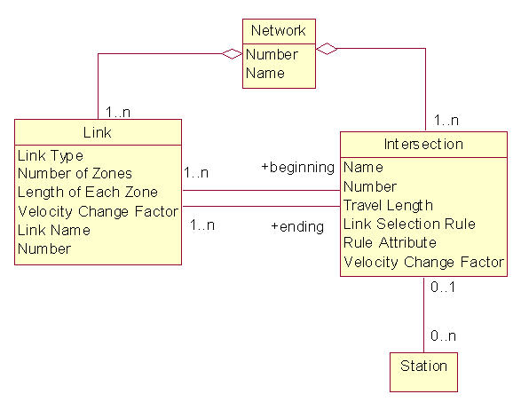
Figure 7.44: Relational diagram for guided vehicle networks
A link is a connection between two points in a network. Every link has a beginning intersection and an ending intersection. The link represents the space between two intersections. The space on the link is divided into an integer number of zones. Each zone has a given length as specified in a consistent unit of measure. All zones have the same length. The link can also be of a certain type (bidirectional, spur, unidirectional). A bidirectional link implies that the transporter is allows to traverse in both directions along the link. A spur is used to model “dead ends,” and unidirectional links restrict traffic to one direction. A velocity change factor can also be associated with a link to indicate a change in the basic velocity of the vehicle while traversing the link. For example, for a link going through an area with many people present, you may want the velocity of the transporter to automatically be reduced. Figure 7.45 illustrates a simple three link network.
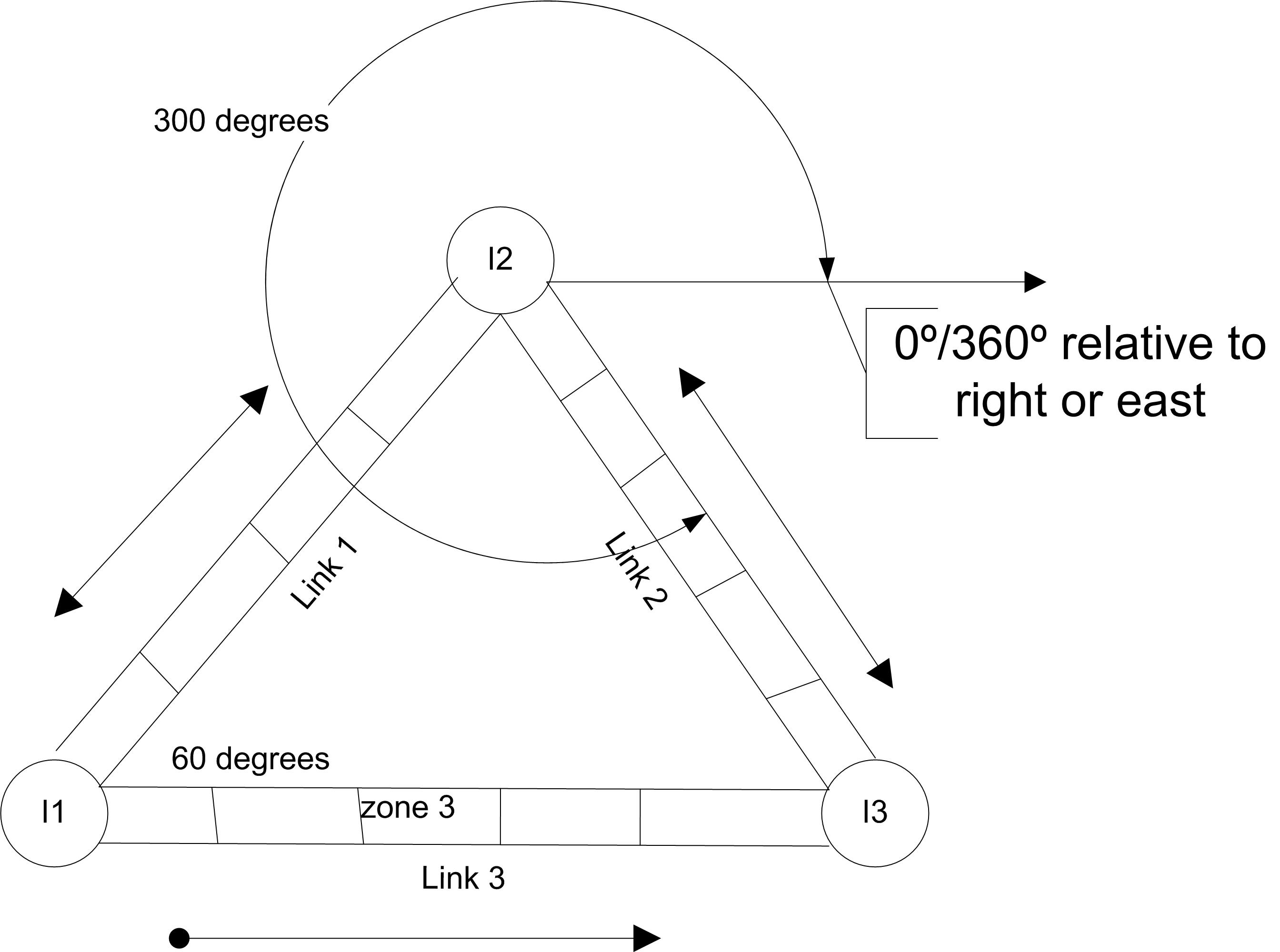
Figure 7.45: Example three link network
In the figure, Link 1 is bidirectional with a beginning intersection
label I1 and an ending intersection labeled I2. Link 1 consists of 4
zones. There can also be a direction of travel specified. The beginning
direction and the ending direction of the link can be used to define the
direction of the link (in degrees) as it leaves the beginning
intersection and as it enters the ending intersection. The direction
entering the ending intersection defaults to the direction leaving the
link’s beginning intersection. Thus, the beginning direction for Link 1
in the figure is 60 degrees. Zero and 360 both represent to the east or
right. The beginning direction for Link 2 is 300 degrees. Think of it
this way, the vehicle has to turn to go onto Link 2. It would have to
turn 60 to get back to zero and then another 60 to head down Link 2.
Since the degrees are specified from the right, this means that the link
2 is 300 degrees relative to an axis going horizontally through
intersection I2. The direction of travel is only relevant if the
acceleration or deceleration of the vehicles as they make turns is
important to the modeling.
In general, an intersection is simply a point in the network; however, the representation of intersections can be more detailed. An intersection also models space: the space between two or more links. Thus, as indicated in Figure 7.44, an intersection may have a length, a velocity change factor, and link selection rule. For more information on the detailed modeling of intersections, you should refer to the INTERSECTIONS element from Arena’s Elements template. Also, the books by Banks et al. (1995) and (Pegden, Shannon, and Sadowski 1995) cover the SIMAN blocks and elements that underlie guided path transporter modeling within . Clearly, a fixed path network consists of a set of links and the associated intersections. Also from Figure 7.44, a station may be associated with an intersection within the network and an intersection may be associated with many stations. Transporters within a guided path network can be sent to specific stations, intersections, or zones. Only the use of stations will be illustrated here.
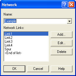
Figure 7.46: NETWORK module for guided path modeling
The new constructs that are to be discussed include the NETWORK and NETWORK LINK modules on the Advanced Transfer template. The NETWORK module allows the user to specify a set of links for a path network. Figure 7.46 shows the NETWORK module. To add links, the user presses the add button or uses the spreadsheet dialog box entry. The links added to the NETWORK module either must already exist or must be edited via the NETWORK LINK module. The NETWORK LINK module permits the definition of the intersections on the links, the directional characteristics of the links, number of zones, zone length, and velocity change factor. Figure 7.47 illustrates the NETWORK LINK module. Notice that the spreadsheet view of the module makes editing multiple links relatively easy.
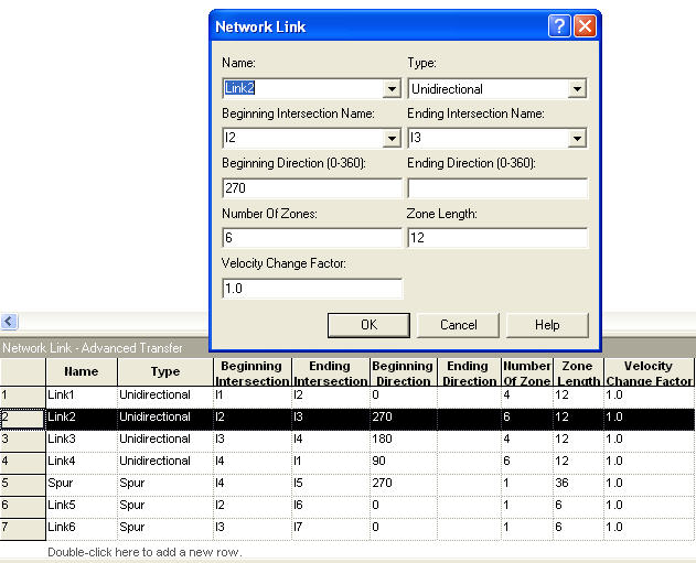
Figure 7.47: NETWORK LINK module
Now, let’s take a look at a simple example. In this example, parts arrive to an entry station every 25 minutes, where they wait for one of two available AGVs. Once loaded onto the AGV (taking 20 minutes) they are transported to the exit station. At the exit station, the item is unloaded, again this takes 20 minutes. The basic layout of the system is shown in Figure 7.48. There are seven intersections and seven links in this example. The distances between the intersections are shown in the figure.
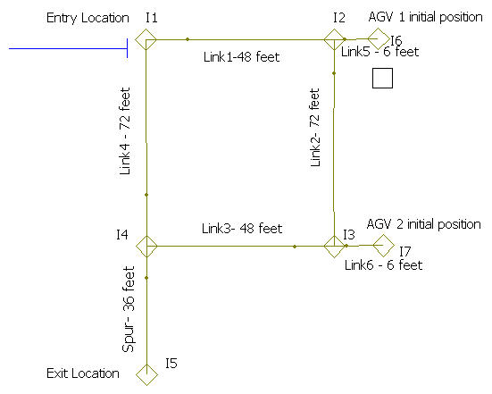
Figure 7.48: Layout for simple AGV example
In modeling this situation, you need to make a number of decisions regarding transporter characteristics, the division of space along the links, the directions of the links, and the zone control of the links. Let’s assume that the item being transported is rather large and heavy. That’s why it takes so long to load and unload. Because of this, the transporter is a cart that is 6 feet in length and only travels 10 feet per minute. There are two carts available for transport. Figure 7.49 shows the TRANSPORTER module for using guided path transporters. When the “Guided” type is selected, additional options become available.
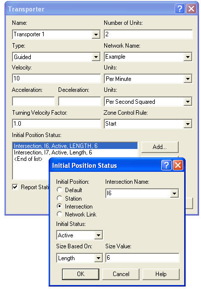
Figure 7.49: TRANSPORTER module for simple AGV example
Because transporters take space on the path, the choice of initial position can be important. A transporter can be placed at a station that has been associated with an intersection, at an intersection, or on a particular zone on a link. The default option will place the transporter at the first network link specified in the NETWORK module associated with the transporter. As long as you place the transporters so that deadlock (to be discussed shortly) does not happen, everything will be fine. In many real systems, the initial location of the vehicles will be obvious. For example, since AGV’s are battery powered they typically have a charging station. Because of this, most systems will be designed with a set of spurs to act as a “home base" for the vehicles. For this simple system, intersections I6 and I7 will be used as the initial position of the transporters. All that is left is to indicate that the transporter is active and specify a length for the transporter of 6 (feet). To be consistent, the velocity is specified as 10 feet per minute. Before discussing the”Zone Control Rule", how to specify the zones for the links needs to be discussed.
Guided path transporters move from zone to zone on the links. The size of the zone, the zone control, and the size of the transporter govern how close the transporters can get to each other while moving. Zones are similar to the cell concept for conveyors. The selection of the size of the zones is really governed by the physical characteristics of the actual system. In this example, assume that the carts should not get too close to each other during movement (perhaps because the big part overhangs the cart). In this example, let’s choose a zone size of 12 feet. Thus, while the cart is in a zone it essentially takes up half of the zone. If you think of the cart as sitting at the midpoint of the zone, then the closest the carts can be is 6 feet (3 feet to the front and 3 feet to the rear).
In Figure 7.47, Link 1 consists of 4 zones of 12 feet in length. Remember the length is whatever unit of measure you want, as long as you are consistent in your specification. With these values, the maximum number of vehicles that could be on Link 1 is four. The rest of the zone specifications are also given in Figure 7.47. Now, you need to decide on the direction of travel permitted on the links. In this system, let’s assume that the AGVs will travel clockwise around the figure. Figure 7.47 indicates that the direction of travel from I1 along Link 1 is zero degrees (to the east). Then, Link 2 has a direction of 270, Link 3 has a direction of 180, and Link 4 has a direction of 90. The spur link to the exit station has a direction of 270 (to the south). Thus, a clockwise turning of the vehicle around the network is achieved. In general, unless you specify the acceleration/deceleration and turning factor for the vehicle, the specification of these directions does not really matter. It has been illustrated here just to indicate what the modeling entails. When working with a real AGV system, these factors can be discerned from the specification of the vehicle and the physical requirements of the system.
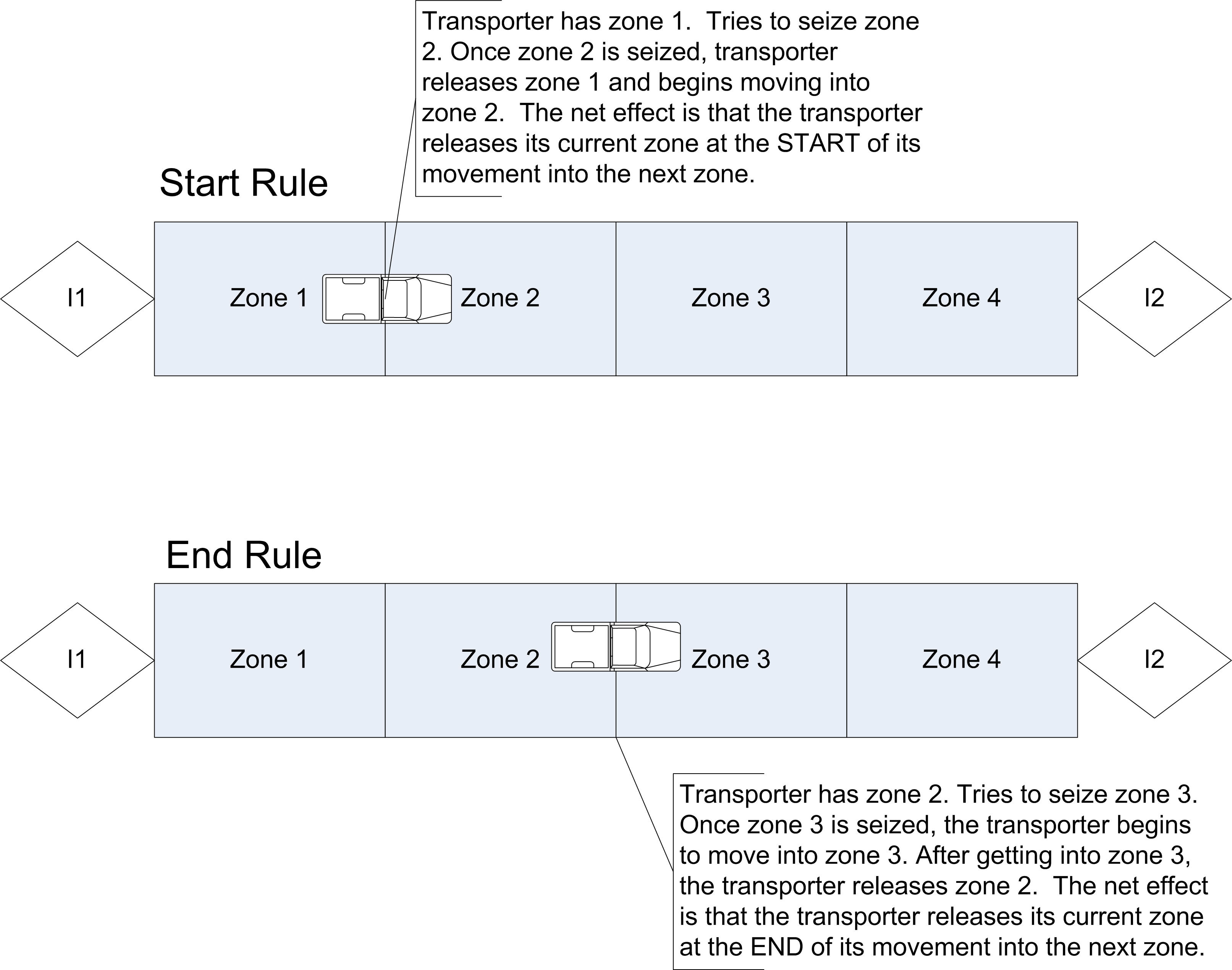
Figure 7.50: Illustrating zone control
To understand why the direction of travel and spurs are important, you need to understand how the transporters move from zone to zone and the concept of deadlock. Zone control governs how the transporter moves from zone to zone. There are three types of control provided by : Start (of next zone), End (of next zone), or distance units k (into next zone). The START rule specifies that the transporter will release its backward most zone when it starts into its next zone. This allows following vehicles to immediately begin to move into the released zone. Figure 7.50 illustrates this concept. In this case, the vehicle is contained in only one zone. In general, a vehicle could cover many zones. The END rule specifies that the transporter will release its backward most zone after it has moved into the next zone (or reached the end of the next zone). This prevents a following vehicle from moving into the transporter’s current zone until it is fully out of the zone. This decision is not critical to most system operations, especially if the vehicle size is specified in terms of zones. The release at end form of control allows for more separation between the vehicles when they are moving. In the distance units k (into next zone) rule, the transporter releases its backward-most zone after traveling the k distance units through the next zone. Since, in general, intersections can be modeled with a traversal distance. These rules also apply to how the vehicles move through intersections and onto links. For more details about the operation of these rules, you should refer to 1 for a discussion of the underlying SIMAN constructs.
As indicated in the zone control discussion, guide path transporters
move by seizing and releasing zones. Now consider the possibility of a
bidirectional link with two transporters moving in opposite directions.
What will happen when the transporters meet? They will crash! No, not
really, but they will cause the system to get in a state of deadlock.
Deadlock occurs when one vehicle requires a zone currently under the
control of a second vehicle, and the second vehicle requires the zone
held by the first vehicle. In some cases, can detect when this occurs
during the simulation run. If it is detected, then will stop with a run
time error. In some cases, cannot detect deadlock. For example, suppose
a station was attached to I4 and a transporter (T1) was sent directly to
that station for some processing. Also, suppose that the part stays on
transporter (T1) during the processing so that transporter (T1) is not
released at the station. Now, suppose that transporter (T2) has just
dropped off something at the exit point, I5, and that a new part has
just come in at I1. Transporter (T2) will want to go through I4 on its
way to I1 to pick up the new part. Transporter (T2) will wait until
transporter (T1) finishes its processing at I4 and if transporter (T1)
eventually moves there will be no problem. However, suppose
transporter (T1) is released at I4 and no other parts arrive for
processing. Transporter (T1) will become idle at the station attached to
I4 and will continue to occupy the space associated with I4. Since, no
arriving parts will ever cause transporter (T1) to move, transporter
(T2) will be stuck. There will be the one part waiting for transporter
(T2), but transporter (T2) will never get there to pick it up.
Obviously, this situation has been concocted to illustrate a possible
undetected deadlock situation. The point is: care must be taken when
designing guided path networks so that deadlock is prevented by design
or that special control logic is added to detect and react to various
deadlock situations. For novice modelers, deadlock can seem troublesome,
especially if you don’t think about where to place the vehicles and if
you have bidirectional links. In most real systems, you should not have
to worry about deadlock because you should design the system not to have
it in the first place! In the simple example, all unidirectional links
were used along with spurs. This prevents many possible deadlock
situations. To illustrate what is meant by design, consider the
concocted undetectable deadlock situation. A simple solution to prevent
it would be to provide a spur for transporter (T1) to receive the
processing that was occurring at the station associated with I4, and
instead associate the processing station with the intersection at the
end of the new spur. Thus, during the processing the vehicle will be out
of the way. If you were designing a real system, wouldn’t you do this
common sense thing anyway? Another simple solution would be to always
send idle vehicles to a staging area or home base that gets them out of
the way of the main path network.
To finish up this discussion, let’s briefly discuss the operation of
spurs and bidirectional links. This discussion is based in part on
(Pegden, Shannon, and Sadowski 1995) page 394. Notice that the link from I4 to I5
is a spur in the previous example. A spur is a special type of link
designed to help prevent some deadlock situations. A spur models a “dead
end” and is bidirectional. If a vehicle is sent to the intersection at
the end of the spur (or to a station attached to the end intersection),
then the vehicle will need to maintain control of the intersection
associated with the entrance to the spur, so that it can get back out.
If the vehicle is too long to fit on the entire spur, then the vehicle
will naturally control the entering intersection. It will block any
vehicles from moving through the intersection. If the spur link is long
enough to accommodate the size of the vehicle, the entering intersection
will be released when the vehicle moves down the spur; however, any
other vehicles that are sent to the end of the spur will not be
permitted to gain access to the entering intersection until all zones in
the spur link are available. This logic only applies to vehicles that
are sent to the end of the spur. Any vehicles sent to or through the
entering intersection of the spur are still permitted to gain access to
the spur’s entering intersection. This allows traffic to continue on the
main path while vehicles are down the spur. Unfortunately, if a vehicle
stops at the entering intersection and then never moves, the situation
described in the concocted example occurs.
Bidirectional links work similarly to unidirectional links, but a vehicle moving on a bidirectional link must have control of both the entering zone on the link and the direction of travel. If another vehicle tries to move on the bidirectional link it must be moving in the same direction as any vehicles currently on the link; otherwise, it will wait. Unfortunately, if a vehicle (wanting to go down a bidirectional link) gains control of the intersection that a vehicle traveling on the bidirectional link needs to exit the link, deadlock may be possible. Because it is so easy to get in deadlock situations with bidirectional links, you should think carefully about their use when using them within your models.
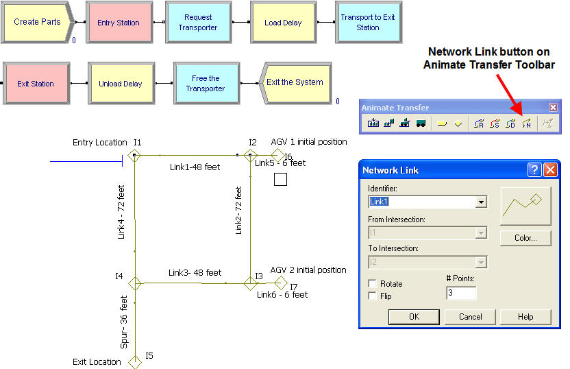
Figure 7.51: Animating guided path transporters
The animation of guided path transporters is very similar to regular transporters. On the Animation Transfer toolbar the Network Link button is used to lay down intersections and the links between the intersections as shown in Figure 7.51. will automatically recognize and fill the pull down text-boxes with the intersections and links that have been defined in the NETWORK LINK module. Although the diagram is not to scale, the rule or scale button comes in very handy when laying out the network links to try to get a good mapping to the physical distances in the problem. Once the network links have been placed, the animation works just like you are used to for transporters. The file, SimpleAGVExample.doe, is available for this problem. In the model, the parts are created and sent to the entry station, where they request a transporter, delay for the loading, and then transport to the exit station. At the exit station, there is a delay for the unloading before the transporter is freed. The REQUEST, TRANSPORT, and FREE modules all work just like for free path transporters.
You should try running the model. You will see that the two transporters start at the specified intersections and you will clearly see the operation of the spur to the exit point as it prevents deadlock. The second transporter will wait for the transporter already on the spur to exit the spur before heading down to the exit point. One useful technique is to use the View \(>\) Layers menu to view the transfer layers during the animation. This will allow the intersections and links to remain visible during the model run.
This section has provided a basic introduction to using guided path transporters in models. There are many more issues related to the use of these constructs that have not been covered:
The construction and use of the shortest path matrix for the guided path network. Since there may be multiple paths through the network, uses standard algorithms to find the shortest path between all intersections in the network. This is used when dispatching the vehicles.
Specialized variables that are used in guided path networks. These variables assist with indicating where the vehicle is within the network, accessing information about the network within the simulation, (e.g. distances, beginning intersection for a link, etc.), status of links, intersections, etc. Arena’s help system under “Transporter Variables” discusses these variables and a discussion of their use can also be found in
Changing of vehicle speeds, handling failures, changing vehicle size, redirecting vehicles through portions of the network, and link selection rules.
More details on these topics can be found in Banks et al. (1995) and 1. Advanced examples are also given in both of those texts, including within 1 the possible use of guided path constructs for modeling automated storage and retrieval systems (AS/RS) and overhead cranes.