8.7 Final Experimental Analysis and Results
While the high capacity system has no problem achieving good system time performance, it will also be the most expensive configuration. Therefore, there is a clear trade off between increased cost and improved customer service. Thus, a system configuration that has the minimum cost while also obtaining desired performance needs to be recommended. This situation can be analyzed in a number of ways using the Process Analyzer and OptQuest within the environment. Often both tools are used to solve the problem. Typically, in an OptQuest analysis, an initial set of screening experiments may be run using the Process Analyzer to get a good idea on the bounds for the problem. Some of this analysis has already been done. See for example Table 8.15. Then, after an OptQuest analysis has been performed, additional experiments might be made via the Process Analyzer to hone the solution space. If only the Process Analyzer is to be used, then a carefully thought out set of experiments can do the job. For teaching purposes, this section will illustrate how to use both the Process Analyzer and OptQuest on this problem.
The contest problem also proposes the use of additional logic to improve the system’s performance on rush samples. In a strict sense, this provides another factor (or design parameter) to consider during the analysis. The inclusion of another factor can dramatically increase the number of experiments to be examined. Because of this, an assumption will be made that the additional logic does not significantly interact with the other factors in the model. If this assumption is true, the original system can be optimized to find a basic design configuration. Then, the additional logic can be analyzed to check if it adds value to the basic solution. In order to recommend a solution, a trade off between cost and system performance must be established. Since the problem specification desires that:
From this simulation study, we would like to know what configuration would provide the most cost-effective solution while achieving high customer satisfaction. Ideally, we would always like to provide results in less time than the contract requires. However, we also do not feel that the system should include extra equipment just to handle the rare occurrence of a late report.
The objective is clear here: minimize total cost. In order to make the occurrence of a late report rare, limits can be set on the probability that the rush and non-rush sample’s system times exceed the contract limits. This can be done by arbitrarily defining rare as 3 out of 100 samples being late. Thus, at least 97% of the non-rush and rush samples must meet the contract requirements.
8.7.1 Using the Process Analyzer on the Problem
This section uses the Process Analyzer on the problem within an experimental design paradigm. Further information on experimental design methods can be found in (Montgomery and Runger 2006). For a discussion of experimental design within a simulation context, please see (Law 2007) or (Kleijnen 1998). There are 6 factors (# units for each of the 5 testing cells and the number of sample holders). To initiate the analysis, a factorial experiment can be used. As shown in Table 8.16, the previously determined resource requirements can be readily used as the low and high settings for the test cells. In addition, the previously determined lower and upper range values for the number of sample holders can be used as the levels for the sample holders.
| Factor | Low | High |
|---|---|---|
| Cell 1 # units | 1 | 2 |
| Cell 2 # units | 1 | 2 |
| Cell 3 # units | 2 | 3 |
| Cell 4 # units | 2 | 4 |
| Cell 5 # units | 3 | 5 |
| # holders | 20 | 36 |
This amounts to \(2^6\) = 64 experiments; however, since sample holders have a cost, it makes sense to first run the half-fraction of the experiment associated with the lower level of the number of holders to see how the test cell resource levels interact. The results for the first half-fraction are shown in Table 8.17. The first readily apparent conclusion that can be drawn from this table is that test cells 1 and 2 must have at least two units of resource capacity. Now, considering cases (2, 2, 2, 4, 5) and (2, 2, 3, 4, 5) it is very likely that test cell # 3 requires 3 units of resource capacity in order to meet the contract requirements. Lastly, it is very clear that the low levels for cell’s 4 and 5 are not acceptable. Thus, the search range can be narrowed down to 3 and 4 units of capacity for cell 4 and to 4 and 5 units of capacity for cell 5.
The other half-fraction with the number of samples at 36 is presented in Table 8.18. The same basic conclusions concerning the resources at the test cells can be made by examining the results. In addition, it is apparent that the number of sample holder can have a significant effect on the performance of the system. It appears that more sample holders hurt the performance of the under capacitated configurations. The effect of the number of sample holders for the highly capacitated systems is some what mixed, but generally the results indicate that 36 sample holders are probably too many for this system. Of course, since this has all been done within an experimental design context, more rigorous statistical tests can be performed to fully test these conclusions. These tests will not do that here, but rather the results will be used to set up another experimental design that can help to better examine the system’s response.
| 1 | 2 | 3 | 4 | 5 | #Holders | Non-Rush | Rush | Time | Cost |
|---|---|---|---|---|---|---|---|---|---|
| 1 | 1 | 2 | 2 | 3 | 20 | 0.000 | 0.963 | 2410.517 | 100340 |
| 2 | 1 | 2 | 2 | 3 | 20 | 0.000 | 0.966 | 2333.135 | 110340 |
| 1 | 2 | 2 | 2 | 3 | 20 | 0.000 | 0.980 | 1913.694 | 112740 |
| 2 | 2 | 2 | 2 | 3 | 20 | 0.000 | 0.973 | 1904.499 | 122740 |
| 1 | 1 | 3 | 2 | 3 | 20 | 0.000 | 0.966 | 2373.574 | 108840 |
| 2 | 1 | 3 | 2 | 3 | 20 | 0.000 | 0.962 | 2407.404 | 118840 |
| 1 | 2 | 3 | 2 | 3 | 20 | 0.000 | 0.973 | 1902.445 | 121240 |
| 2 | 2 | 3 | 2 | 3 | 20 | 0.000 | 0.978 | 1865.821 | 131240 |
| 1 | 1 | 2 | 4 | 3 | 20 | 0.000 | 0.951 | 2332.412 | 119940 |
| 2 | 1 | 2 | 4 | 3 | 20 | 0.000 | 0.949 | 2365.047 | 129940 |
| 1 | 2 | 2 | 4 | 3 | 20 | 0.003 | 0.985 | 496.292 | 132340 |
| 2 | 2 | 2 | 4 | 3 | 20 | 0.025 | 0.986 | 284.205 | 142340 |
| 1 | 1 | 3 | 4 | 3 | 20 | 0.000 | 0.956 | 2347.050 | 128440 |
| 2 | 1 | 3 | 4 | 3 | 20 | 0.000 | 0.956 | 2316.931 | 138440 |
| 1 | 2 | 3 | 4 | 3 | 20 | 0.019 | 0.984 | 364.081 | 140840 |
| 2 | 2 | 3 | 4 | 3 | 20 | 0.122 | 0.987 | 157.798 | 150840 |
| 1 | 1 | 2 | 2 | 5 | 20 | 0.000 | 0.968 | 2394.530 | 122740 |
| 2 | 1 | 2 | 2 | 5 | 20 | 0.000 | 0.965 | 2360.751 | 132740 |
| 1 | 2 | 2 | 2 | 5 | 20 | 0.000 | 0.980 | 1873.405 | 135140 |
| 2 | 2 | 2 | 2 | 5 | 20 | 0.000 | 0.982 | 1865.020 | 145140 |
| 1 | 1 | 3 | 2 | 5 | 20 | 0.000 | 0.963 | 2391.649 | 131240 |
| 2 | 1 | 3 | 2 | 5 | 20 | 0.000 | 0.965 | 2361.708 | 141240 |
| 1 | 2 | 3 | 2 | 5 | 20 | 0.000 | 0.974 | 1926.889 | 143640 |
| 2 | 2 | 3 | 2 | 5 | 20 | 0.000 | 0.980 | 1841.387 | 153640 |
| 1 | 1 | 2 | 4 | 5 | 20 | 0.000 | 0.951 | 2387.810 | 142340 |
| 2 | 1 | 2 | 4 | 5 | 20 | 0.000 | 0.955 | 2352.933 | 152340 |
| 1 | 2 | 2 | 4 | 5 | 20 | 0.202 | 0.986 | 121.199 | 154740 |
| 2 | 2 | 2 | 4 | 5 | 20 | 0.683 | 0.991 | 43.297 | 164740 |
| 1 | 1 | 3 | 4 | 5 | 20 | 0.000 | 0.954 | 2291.880 | 150840 |
| 2 | 1 | 3 | 4 | 5 | 20 | 0.000 | 0.947 | 2332.031 | 160840 |
| 1 | 2 | 3 | 4 | 5 | 20 | 0.439 | 0.985 | 69.218 | 163240 |
| 2 | 2 | 3 | 4 | 5 | 20 | 0.961 | 0.991 | 21.431 | 173240 |
| 1 | 2 | 3 | 4 | 5 | #Holders | Non-Rush | Rush | Time | Cost |
|---|---|---|---|---|---|---|---|---|---|
| 1 | 1 | 2 | 2 | 3 | 36 | 0.000 | 0.776 | 2319.323 | 106532 |
| 2 | 1 | 2 | 2 | 3 | 36 | 0.000 | 0.764 | 2260.829 | 116532 |
| 1 | 2 | 2 | 2 | 3 | 36 | 0.000 | 0.729 | 1816.568 | 118932 |
| 2 | 2 | 2 | 2 | 3 | 36 | 0.000 | 0.714 | 1779.530 | 128932 |
| 1 | 1 | 3 | 2 | 3 | 36 | 0.000 | 0.768 | 2238.654 | 115032 |
| 2 | 1 | 3 | 2 | 3 | 36 | 0.000 | 0.775 | 2243.560 | 125032 |
| 1 | 2 | 3 | 2 | 3 | 36 | 0.000 | 0.730 | 1762.579 | 127432 |
| 2 | 2 | 3 | 2 | 3 | 36 | 0.000 | 0.717 | 1763.306 | 137432 |
| 1 | 1 | 2 | 4 | 3 | 36 | 0.000 | 0.796 | 2244.243 | 126132 |
| 2 | 1 | 2 | 4 | 3 | 36 | 0.000 | 0.790 | 2268.549 | 136132 |
| 1 | 2 | 2 | 4 | 3 | 36 | 0.202 | 0.900 | 111.232 | 138532 |
| 2 | 2 | 2 | 4 | 3 | 36 | 0.385 | 0.915 | 72.860 | 148532 |
| 1 | 1 | 3 | 4 | 3 | 36 | 0.000 | 0.806 | 2255.190 | 134632 |
| 2 | 1 | 3 | 4 | 3 | 36 | 0.000 | 0.795 | 2251.548 | 144632 |
| 1 | 2 | 3 | 4 | 3 | 36 | 0.360 | 0.899 | 76.398 | 147032 |
| 2 | 2 | 3 | 4 | 3 | 36 | 0.405 | 0.911 | 68.676 | 157032 |
| 1 | 1 | 2 | 2 | 5 | 36 | 0.000 | 0.771 | 2304.784 | 128932 |
| 2 | 1 | 2 | 2 | 5 | 36 | 0.000 | 0.771 | 2250.198 | 138932 |
| 1 | 2 | 2 | 2 | 5 | 36 | 0.000 | 0.738 | 1753.819 | 141332 |
| 2 | 2 | 2 | 2 | 5 | 36 | 0.000 | 0.717 | 1751.676 | 151332 |
| 1 | 1 | 3 | 2 | 5 | 36 | 0.000 | 0.780 | 2251.174 | 137432 |
| 2 | 1 | 3 | 2 | 5 | 36 | 0.000 | 0.771 | 2252.106 | 147432 |
| 1 | 2 | 3 | 2 | 5 | 36 | 0.000 | 0.726 | 1781.024 | 149832 |
| 2 | 2 | 3 | 2 | 5 | 36 | 0.000 | 0.716 | 1794.930 | 159832 |
| 1 | 1 | 2 | 4 | 5 | 36 | 0.000 | 0.787 | 2243.338 | 148532 |
| 2 | 1 | 2 | 4 | 5 | 36 | 0.000 | 0.794 | 2243.558 | 158532 |
| 1 | 2 | 2 | 4 | 5 | 36 | 0.541 | 0.897 | 54.742 | 160932 |
| 2 | 2 | 2 | 4 | 5 | 36 | 0.898 | 0.932 | 28.974 | 170932 |
| 1 | 1 | 3 | 4 | 5 | 36 | 0.000 | 0.791 | 2263.484 | 157032 |
| 2 | 1 | 3 | 4 | 5 | 36 | 0.000 | 0.799 | 2278.707 | 167032 |
| 1 | 2 | 3 | 4 | 5 | 36 | 0.604 | 0.884 | 49.457 | 169432 |
| 2 | 2 | 3 | 4 | 5 | 36 | 0.994 | 0.983 | 16.588 | 179432 |
Using the initial results in Table 8.15 and the analysis of the two half-fraction experiments, another set of experiments were designed to focus in on the capacities for cells 3, 4, and 5. The experiments are given in Table 8.19. This set of experiments is a \(2^4\) = 16 factorial experiment. The results are shown in Table 8.20. The results have been sorted such that the systems that have the higher chance of meeting the contract requirements are at the top of the table. From the results, it should be clear that cell 3 requires at least 3 units of capacity for the system to be able to meet the requirements. It is also very likely that cell 4 requires 4 testers to meet the requirements. Thus, the search space has been narrowed to either 4 or 5 testers at cell 5 and between 20 and 24 holders.
| Factor | Low | High |
|---|---|---|
| Cell 3 # units | 2 | 3 |
| Cell 4 # units | 3 | 4 |
| Cell 5 # units | 4 | 5 |
| # holders | 20 | 24 |
| 1 | 2 | 3 | 4 | 5 | #Holders | Non-Rush | Rush | Time | Cost |
|---|---|---|---|---|---|---|---|---|---|
| 2 | 2 | 3 | 4 | 5 | 24 | 0.988 | 0.990 | 16.355 | 174788 |
| 2 | 2 | 3 | 4 | 4 | 24 | 0.970 | 0.988 | 19.410 | 163588 |
| 2 | 2 | 3 | 4 | 5 | 20 | 0.961 | 0.991 | 21.431 | 173240 |
| 2 | 2 | 3 | 4 | 4 | 20 | 0.945 | 0.989 | 25.270 | 162040 |
| 2 | 2 | 3 | 3 | 4 | 24 | 0.877 | 0.987 | 30.345 | 153788 |
| 2 | 2 | 3 | 3 | 5 | 24 | 0.871 | 0.988 | 31.244 | 164988 |
| 2 | 2 | 2 | 4 | 5 | 24 | 0.812 | 0.984 | 34.065 | 166288 |
| 2 | 2 | 2 | 4 | 4 | 24 | 0.782 | 0.986 | 35.289 | 155088 |
| 2 | 2 | 3 | 3 | 5 | 20 | 0.734 | 0.991 | 39.328 | 163440 |
| 2 | 2 | 3 | 3 | 4 | 20 | 0.731 | 0.992 | 40.370 | 152240 |
| 2 | 2 | 2 | 3 | 4 | 24 | 0.687 | 0.987 | 42.891 | 145288 |
| 2 | 2 | 2 | 4 | 5 | 20 | 0.683 | 0.991 | 43.297 | 164740 |
| 2 | 2 | 2 | 3 | 5 | 24 | 0.656 | 0.980 | 46.049 | 156488 |
| 2 | 2 | 2 | 4 | 4 | 20 | 0.627 | 0.989 | 45.708 | 153540 |
| 2 | 2 | 2 | 3 | 5 | 20 | 0.561 | 0.987 | 52.710 | 154940 |
| 2 | 2 | 2 | 3 | 4 | 20 | 0.492 | 0.985 | 59.671 | 143740 |
To finalize the selection of the best configuration for the current situation, ten experimental combinations of cell 5 resource capacity (4, 5) and number of sample holders (20, 21, 22, 23, 24) were run in the Process Analyzer using 10 replications for each scenario. The results of the experiments are shown in Table 8.21. In addition, the multiple comparison procedure was applied to the results based on picking the solution with the best (highest) non-rush probability. The results of that comparison are shown in Figure 8.31. The multiple comparison procedure indicates with 95% confidence that scenarios 3, 4, 5, 7, 8, 9, 10 are the best. Since there is essentially no difference between them, the cheapest configuration can be chosen, which is scenario 3 with factor levels of (2, 3, 3, 4, 4, and 22) and a total cost of $162, 814.
Based on the results of this section, a solid solution for the problem has been determined; however, to give you experience applying OptQuest to a problem, let us examine its application to this situation.
| Scenario | 1 | 2 | 3 | 4 | 5 | #Holders | Non-Rush | Rush | Time | Cost |
|---|---|---|---|---|---|---|---|---|---|---|
| 1 | 2 | 2 | 3 | 4 | 4 | 20 | 0.917 | 0.987 | 26.539 | 162040 |
| 2 | 2 | 2 | 3 | 4 | 4 | 21 | 0.942 | 0.987 | 23.273 | 162427 |
| 3 | 2 | 2 | 3 | 4 | 4 | 22 | 0.976 | 0.989 | 20.125 | 162814 |
| 4 | 2 | 2 | 3 | 4 | 4 | 23 | 0.974 | 0.988 | 19.983 | 163201 |
| 5 | 2 | 2 | 3 | 4 | 4 | 24 | 0.979 | 0.989 | 18.512 | 163588 |
| 6 | 2 | 2 | 3 | 4 | 5 | 20 | 0.958 | 0.988 | 21.792 | 173240 |
| 7 | 2 | 2 | 3 | 4 | 5 | 21 | 0.967 | 0.987 | 19.362 | 173627 |
| 8 | 2 | 2 | 3 | 4 | 5 | 22 | 0.984 | 0.988 | 18.022 | 174014 |
| 9 | 2 | 2 | 3 | 4 | 5 | 23 | 0.986 | 0.988 | 16.971 | 174401 |
| 10 | 2 | 2 | 3 | 4 | 5 | 24 | 0.980 | 0.987 | 16.996 | 174788 |
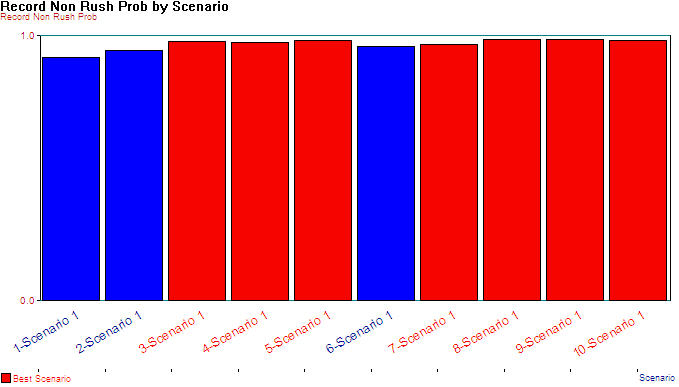
Figure 8.31: Multiple comparison results for non-rush probability
8.7.2 Using OptQuest on the Problem
OptQuest is an add-on program for Arena which provides heuristic based simulation optimization capabilities. You can find OptQuest on Tools \(>\) OptQuest. OptQuest will open up and you should see a dialog asking you whether you want to browse for an already formulated optimization run or to start a new optimization run. Select the start new optimization run button. OptQuest will then read your model and start a new optimization model, which may take a few seconds, depending on the size of your model. OptQuest is similar to the Process Analyzer in some respects. It allows you to define controls and responses for your model. Then you can develop an optimization function that will be used to evaluate the system under the various controls. In addition, you can define a set of constraints that must not be violated by the final recommended solution to the optimization model. It is beyond the scope of this example to fully describe simulation optimization and all the intricacies of this technology. The interested reader should refer to April et al. (2001) and Glover, Kelly, and Laguna (1999) for more information on this technology. This example will simply illustrate the possibilities of using this technology. A tutorial on the use of OptQuest is available in the OptQuest help files.
As shown in Figure 8.32, OptQuest for can be used to define controls and responses and to setup an optimization model to minimize total cost subject to the probability of non-rush and rush samples meeting the contract requirements being greater than or equal to 0.97. When running OptQuest, it is a good idea to try to give OptQuest a good starting point. Since the high resource case is already known to be feasible from the pilot experiments, the optimization can be started using the high resource case and the number of sample holders within the middle of their range (e.g. 27 sample holders).
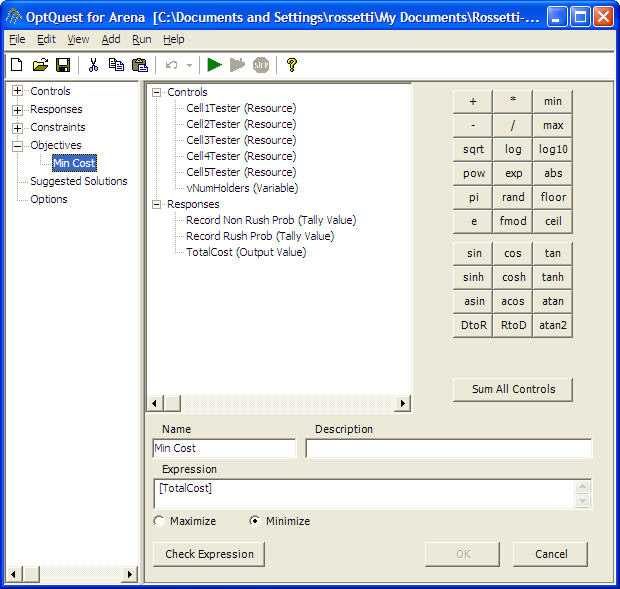
Figure 8.32: Defining the objective function in OptQuest
The simulation optimization was executed over a period of about 6 hours (wall clock time) until it was manually stopped after 79 total simulations. From Figure 8.33, the best solution was 2 testers at cells 1 and 2, 3 testers at cell 3, 4 testers at cells 4 and 5, and 23 sample holders. The total cost of this configuration is $163, 201. This solution has 1 more sample holder as compared to the solution based on the Process Analyzer. Of course, you would not know this if the analysis was based solely on OptQuest. OptQuest allows top solutions to be saved to a file. Upon looking at those solutions it becomes clear that the heuristic in OptQuest has found the basic configuration for the test cells (2, 2, 3, 4, 4) and is investigating the number of sample holders. If the optimization had been allowed to run longer it is very likely that it would have recommended 22 sample holders. At this stage, the Process Analyzer can be used to hone in on the recommended OptQuest solution by more closely examining the final set of “best” solutions. Since that has already been done in the previous section, it will not be included here.
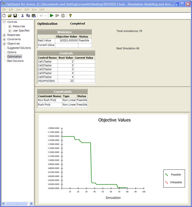
Figure 8.33: Results from the OptQuest run
8.7.3 Investigating the New Logic Alternative
Now that a recommended basic configuration is available, the alternative logic needs to be checked to see if it can improve performance for the additional cost. In addition, the suggested number for the control logic should be determined. The basic model can be easily modified to contain the alternative logic. This was done within the load/unload sub-model. In addition, a flag variable was used to be able to turn on or turn off the use of the new logic so that the Process Analyzer can control whether or not the logic is included in the model. The implementation can be found in the file, SMTesting.doe.
To reduce the number of factors involved in the previous analysis, it was assumed that the new logic did not interact significantly with the allocation of the test cell capacity; however, because the suggested number checks for how many samples are waiting at the load/unload station, there may be some interaction between these factors. Based on these assumptions, 10 scenarios with the new logic were designed for the recommended tester configuration (2, 2, 3, 4, 4) varying the number of holders between 20 and 24 with the suggested number (SN) set at both 2 and 3. TTable 8.22 presents the results of these experiments. From the results, it is clear that the new logic does not have a substantial impact on the probability of meeting the contract for the non-rush and rush samples. In fact, looking at scenario 3, the new logic may actually hurt the non-rush samples. To complete the analysis, a more rigorous statistical comparison should be performed; however, that task will be skipped for the sake of brevity.
| Scenario | 1 | 2 | 3 | 4 | 5 | #Holders | SN | Non-Rush | Rush | Time |
|---|---|---|---|---|---|---|---|---|---|---|
| 1 | 2 | 2 | 3 | 4 | 4 | 20 | 2 | 0.937 | 0.989 | 23.937 |
| 2 | 2 | 2 | 3 | 4 | 4 | 21 | 2 | 0.956 | 0.988 | 21.461 |
| 3 | 2 | 2 | 3 | 4 | 4 | 22 | 2 | 0.957 | 0.989 | 21.159 |
| 4 | 2 | 2 | 3 | 4 | 4 | 23 | 2 | 0.972 | 0.989 | 19.011 |
| 5 | 2 | 2 | 3 | 4 | 4 | 24 | 2 | 0.975 | 0.986 | 18.665 |
| 6 | 2 | 2 | 3 | 4 | 4 | 20 | 3 | 0.926 | 0.989 | 25.305 |
| 7 | 2 | 2 | 3 | 4 | 4 | 21 | 3 | 0.948 | 0.988 | 22.449 |
| 8 | 2 | 2 | 3 | 4 | 4 | 22 | 3 | 0.968 | 0.989 | 20.536 |
| 9 | 2 | 2 | 3 | 4 | 4 | 23 | 3 | 0.983 | 0.988 | 18.591 |
| 10 | 2 | 2 | 3 | 4 | 4 | 24 | 3 | 0.986 | 0.987 | 18.170 |
After all the analysis, the results indicate that SMTesting should proceed with the (2, 2, 3, 4, 4) configuration with 22 sample holders for a total cost of $162, 814. The additional one-time purchase of the control logic is not warranted at this time.
8.7.4 Sensitivity Analysis
This realistically sized case study clearly demonstrates the application of simulation to designing a manufacturing system. The application of simulation was crucial in this analysis because of the complex, dynamic relationships between the elements of the system and because of the inherent stochastic environment (e.g. arrivals, breakdowns, etc.) that were in the problem. Based on the analysis performed for the case study, SMTesting should be confident that the recommended design will suffice for the current situation. However, there are a number of additional steps that can (and probably should) be performed for the problem.
In particular, to have even more confidence in the design, simulation offers the ability to perform a sensitivity analysis on the "uncontrollable" factors in the environment. While the analysis in the previous section concentrated on the design parameters that can be controlled, it is very useful to examine the sensitivity of other factors and assumptions on the recommended solution. Now that a verified and validated model is in place, the arrival rates, the breakdown rates, repair times, the buffer sizes, etc. can all be varied to see how they affect the recommendation. In addition, a number of explicit and implicit assumptions were made during the modeling and analysis of the contest problem. For example, when modeling the breakdowns of the testers, the FAILURE module was used. This module assumes that when a failure occurs that all units of the resource become failed. This may not actually be the case. In order to model individual unit failures, the model must be modified. After the modification, the assumption can be tested to see if it makes a difference with respect to the recommended solution. Other aspects of the situation were also omitted. For example, the fact that tests may have to be repeated at test cells was left out due to the fact that no information was given as to the likelihood for repeating the test. This situation could be modeled and a re-test probability assumed. Then, the sensitivity to this assumption could be examined.
In addition to modeling assumptions, assumptions were made during the experimental analysis. For example, basic resource configuration of (2, 2, 3, 4, 4) was assumed to not change if the control logic was introduced. This can also be tested within a sensitivity analysis. Since performing a sensitivity analysis has been discussed in previously in this chapter the mechanics of performing sensitivity analysis will not be discussed here. A number of exercises will ask you to explore these issues.