A.2 Generating Random Variates from Distributions
In simulation, pseudo random numbers serve as the foundation for generating samples from probability distribution models. We will now assume that the random number generator has been rigorously tested and that it produces sequences of \(U_{i} \sim U(0,1)\) numbers. We now want to take the \(U_{i} \sim U(0,1)\) and utilize them to generate from probability distributions.
The realized value from a probability distribution is called a random variate. Simulations use many different probability distributions as inputs. Thus, methods for generating random variates from distributions are required. Different distributions may require different algorithms due to the challenges of efficiently producing the random variables. Therefore, we need to know how to generate samples from probability distributions. In generating random variates the goal is to produce samples \(X_{i}\) from a distribution \(F(x)\) given a source of random numbers, \(U_{i} \sim U(0,1)\). There are four basic strategies or methods for producing random variates:
- Inverse transform or inverse cumulative distribution function (CDF) method
- Convolution
- Acceptance/Rejection
- Mixture and Truncated Distributions
The following sections discuss each of these methods.
A.2.1 Inverse Transform Method
The inverse transform method is the preferred method for generating random variates provided that the inverse transform of the cumulative distribution function can be easily derived or computed numerically. The key advantage for the inverse transform method is that for every \(U_{i}\) use a corresponding \(X_{i}\) will be generated. That is, there is a one-to-one mapping between the pseudo-random number \(u_i\) and the generated variate \(x_i\).
The inverse transform technique utilizes the inverse of the cumulative distribution function as illustrated in Figure A.2, will illustrates simple cumulative distribution function. First, generate a number, \(u_{i}\) between 0 and 1 (along the \(U\) axis), then find the corresponding \(x_{i}\) coordinate by using \(F^{-1}(\cdot)\). For various values of \(u_{i}\), the \(x_{i}\) will be properly ‘distributed’ along the x-axis. The beauty of this method is that there is a one to one mapping between \(u_{i}\) and \(x_{i}\). In other words, for each \(u_{i}\) there is a unique \(x_{i}\) because of the monotone property of the CDF.
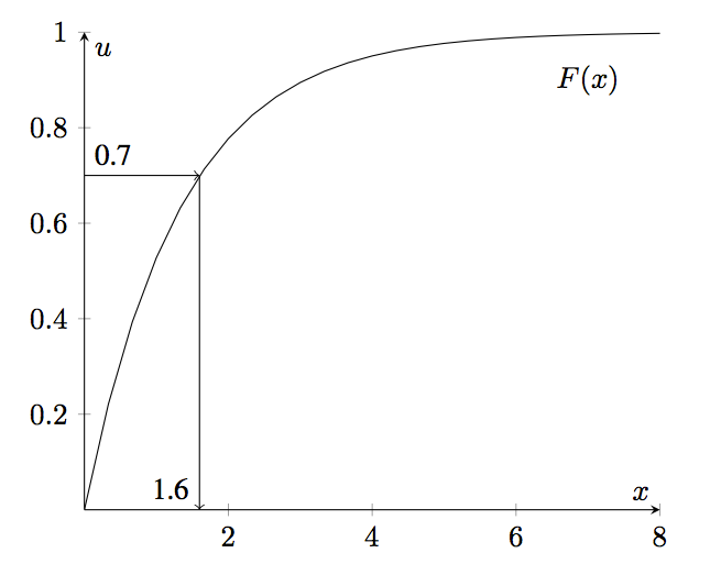
Figure A.2: Inverse Transform Method
The idea illustrated in Figure A.2 is based on the following theorem.
The proof utilizes the definition of the cumulative distribution function to derive the CDF for \(Y\).
\[ \begin{split} F(y) & = P\left\{Y \leq y \right\} \\ & = P\left\{F(X) \leq y\right\} \; \text{substitute for } Y \\ & = P\left\{F^{-1}(F(X)) \leq F^{-1}(y)\right\} \; \text{apply inverse} \\ & = P\left\{X \leq F^{-1}(y)\right\} \; \text{definition of inverse} \\ & = F(F^{-1}(y)) \; \text{definition of CDF}\\ & = y \; \text{definition of inverse} \end{split} \] Since \(P(Y \leq y) = y\) defines a \(U(0,1)\) random variable, the proof is complete.
This result also works in reverse if you start with a uniformly distributed random variable then you can get a random variable with the distribution of \(F(x)\). The idea is to generate \(U_{i} \sim U(0,1)\) and then to use the inverse cumulative distribution function to transform the random number to the appropriately distributed random variate.
Let’s assume that we have a function, randU01(), that will provide pseudo-random numbers on the range (0,1). Then, the following presents the pseudo-code for the inverse transform algorithm.
2. \(x = F^{-1}(u)\)
3. return \(x\)
Line 1 generates a uniform number. Line 2 takes the inverse of \(u\) and line 3 returns the random variate. The following example illustrates the inverse transform method for the exponential distribution.
The exponential distribution is often used to model the time until and event (e.g. time until failure, time until an arrival etc.) and has the following probability density function:
\[ f(x) = \begin{cases} 0.0 & \text{if} \left\{x < 0\right\}\\ \lambda e^{-\lambda x} & \text{if} \left\{x \geq 0 \right\} \\ \end{cases} \] with \[ \begin{split} E\left[X\right] &= \frac{1}{\lambda} \\ Var\left[X\right] &= \frac{1}{\lambda^2} \end{split} \]
Solution for Example A.2 In order to solve this problem, we must first compute the CDF for the exponential distribution. For any value, \(b < 0\), we have by definition:
\[ F(b) = P\left\{X \le b \right\} = \int_{ - \infty }^b f(x)\;dx = \int\limits_{ - \infty }^b {0 dx} = 0 \] For any value \(b \geq 0\),
\[ \begin{split} F(b) & = P\left\{X \le b \right\} = \int_{ - \infty }^b f(x)dx\\ & = \int_{ - \infty }^0 f(x)dx + \int\limits_0^b f(x)dx \\ & = \int\limits_{0}^{b} \lambda e^{\lambda x}dx = - \int\limits_{0}^{b} e^{-\lambda x}(-\lambda)dx\\ & = -e^{-\lambda x} \bigg|_{0}^{b} = -e^{-\lambda b} - (-e^{0}) = 1 - e^{-\lambda b} \end{split} \] Thus, the CDF of the exponential distribution is: \[ F(x) = \begin{cases} 0 & \text{if} \left\{x < 0 \right\}\\ 1 - e^{-\lambda x} & \text{if} \left\{x \geq 0\right\}\\ \end{cases} \] Now the inverse of the CDF can be derived by setting \(u = F(x)\) and solving for \(x = F^{-1}(u)\).
\[ \begin{split} u & = 1 - e^{-\lambda x}\\ x & = \frac{-1}{\lambda}\ln \left(1-u \right) = F^{-1}(u) \end{split} \] For Example A.2, we have that \(E[X]= 1.\overline{33}\). Since \(E\left[X\right] = 1/\lambda\) for the exponential distribution, we have that \(\lambda = 0.75\). Since \(u=0.7\), then the generated random variate, \(x\), would be:
\[x = \frac{-1}{0.75}\ln \left(1-0.7 \right) = 1.6053\] Thus, if we let \(\theta = E\left[X\right]\), the formula for generating an exponential random variate is simply:
\[\begin{equation} x = \frac{-1}{\lambda}\ln \left(1-u \right) = -\theta \ln{(1-u)} \tag{A.1} \end{equation}\]
In the following pseudo-code, we assume that randU01() is a function that returns a uniformly distributed random number over the range (0,1).
2. \(x = \frac{-1}{\lambda}\ln \left(1-u \right)\)
3. return \(x\)
Thus, the key to applying the inverse transform technique for generating random variates is to be able to first derive the cumulative distribution function (CDF) and then to derive its inverse function. It turns out that for many common distributions, the CDF and inverse CDF well known.
The uniform distribution over an interval \((a,b)\) is often used to model situations where the analyst does not have much information and can only assume that the outcome is equally likely over a range of values. The uniform distribution has the following characteristics:
\[X \sim \operatorname{Uniform}(a,b)\] \[ f(x) = \begin{cases} \frac{1}{b-a } & a \leq x \leq b\\ 0 & \text{otherwise} \end{cases} \] \[ \begin{split} E\left[X\right] &= \frac{a+b}{2}\\ Var\left[X\right] &= \frac{(b-a)^{2}}{12} \end{split} \]
\[ F(x) = \begin{cases} 0.0 & x < a\\ \frac{x-a}{b-a} & a \leq x \leq b\\ 1.0 & x > b \end{cases} \]
Solution for Example A.3 To solve this problem, we must determine the inverse CDF algorithm for the \(U(a,b)\) distribution. The inverse of the CDF can be derived by setting \(u = F(x)\) and solving for \(x = F^{-1}(u)\). \[ \begin{split} u & = \frac{x-a}{b-a}\\ u(b-a) &= x-a \\ x & = a + u(b-a) = F^{-1}(u) \end{split} \] For the example, we have that \(a = 5\) and \(b = 35\) and \(u=0.25\), then the generated \(x\) would be:
\[ F^{-1}(u) = x = 5 + 0.25\times(35 - 5) = 5 + 7.5 = 12.5 \] Notice how the value of \(u\) is first scaled on the range \((0,b-a)\) and then shifted to the range \((a, b)\). For the uniform distribution this transformation is linear because of the form of its \(F(x)\).
2. \(x = a + u(b-a)\)
3. return \(x\)
For the previous distributions a closed form representation of the cumulative distribution function was available. If the cumulative distribution function can be inverted, then the inverse transform method can be easily used to generate random variates from the distribution. If no closed form analytical formula is available for the inverse cumulative distribution function, then often we can resort to numerical methods to implement the function. For example, the normal distribution is an extremely useful distribution and numerical methods have been devised to provide its inverse cumulative distribution function.
The inverse CDF method also works for discrete distributions. For a discrete random variable, \(X\), with possible values \(x_1, x_2, \ldots, x_n\) (\(n\) may be infinite), the probability distribution is called the probability mass function (PMF) and denoted:
\[ f\left( {{x_i}} \right) = P\left( {X = {x_i}} \right) \]
where \(f\left( {{x_i}} \right) \ge 0\) for all \({x_i}\) and
\[ \sum\limits_{i = 1}^n {f\left({{x_i}} \right)} = 1 \]
The cumulative distribution function is
\[ F(x) = P\left( {X \le x} \right) = \sum\limits_{{x_i} \le x} {f\left( {{x_i}} \right)} \] and satisfies, \(0 \le F\left( x \right) \le 1\), and if \(x \le y\) then \(F(x) \le F(y)\).
In order to apply the inverse transform method to discrete distributions, the cumulative distribution function can be searched to find the value of \(x\) associated with the given \(u\). This process is illustrated in the following example.
| \(x_{i}\) | 1 | 2 | 3 | 4 |
|---|---|---|---|---|
| \(f(x_{i})\) | 0.4 | 0.3 | 0.2 | 0.1 |
Plot the probability mass function and cumulative distribution function for this random variable. Then, develop an inverse cumulative distribution function for generating from this distribution. Finally, given \(u_1 = 0.934\) and \(u_2 = 0.1582\) are pseudo-random numbers, generate the two corresponding random variates from this PMF.
Solution for Example A.4 To solve this example, we must understand the functional form of the PMF and CDF, which are given as follows:
\[ P\left\{X=x\right\} = \begin{cases} 0.4 & \text{x = 1}\\ 0.3 & \text{x = 2}\\ 0.2 & \text{x = 3}\\ 0.1 & \text{x = 4} \end{cases} \]
\[ F(x) = \begin{cases} 0.0 & \text{if} \; x < 1\\ 0.4 & \text{if} \; 1 \le x < 2\\ 0.7 & \text{if} \; 2 \le x < 3\\ 0.9 & \text{if} \; 3 \le x < 4\\ 1.0 & \text{if} \; x \geq 4 \end{cases} \]
Figure A.3 illustrates the CDF for this discrete distribution.
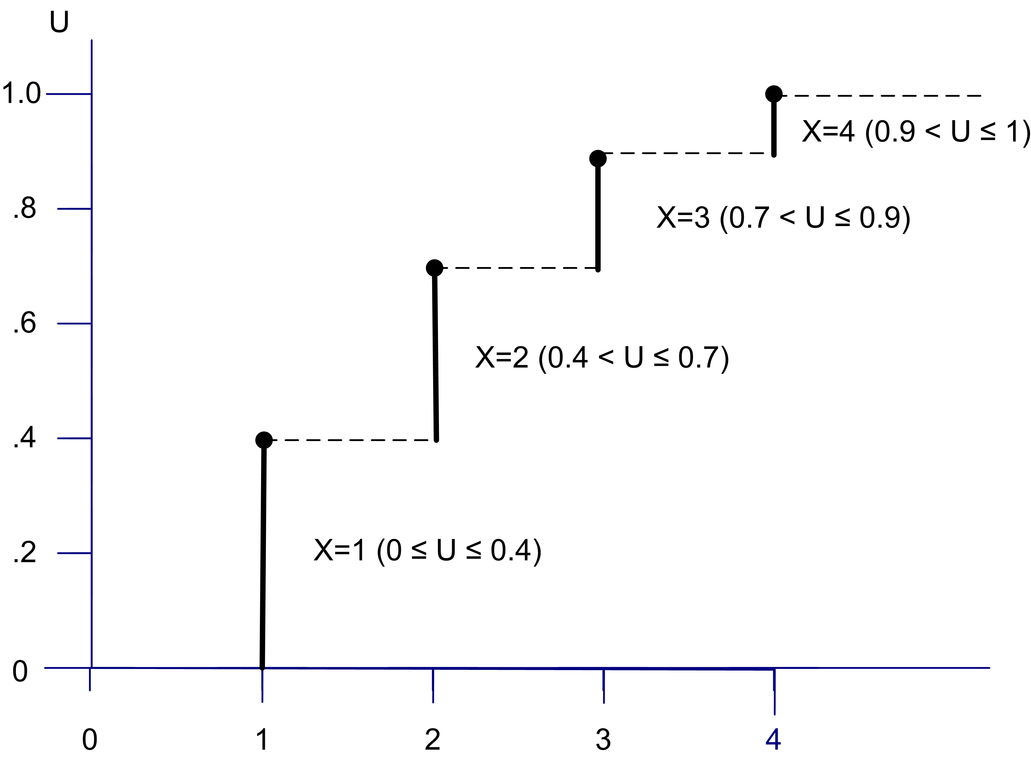
Figure A.3: Example Empirical CDF
Examining Figure A.3 indicates that for any value of \(u_{i}\) in the interval, \(\left(0.4, 0.7\right]\) you get an \(x_{i}\) of 2. Thus, generating random numbers from this distribution can be accomplished by using the inverse of the cumulative distribution function.
\[ F^{-1}(u) = \begin{cases} 1 & \text{if} \; 0.0 \leq u \leq 0.4\\ 2 & \text{if} \; 0.4 < u \leq 0.7 \\ 3 & \text{if} \; 0.7 < u \leq 0.9\\ 4 & \text{if} \; 0.9 < u \leq 1.0\\ \end{cases} \]
Suppose \(u_1 = 0.934\), then by \(F^{-1}(u)\), \(x = 4\). If \(u_2 = 0.1582\), then \(x = 1\). Thus, we use the inverse transform function to look up the appropriate \(x\) for a given \(u\).
For a discrete distribution, given a value for \(u\), pick \(x_{i}\), such that \(F(x_{i-1}) < u \leq F(x_{i})\) provides the inverse CDF function. Thus, for any given value of \(u\) the generation process amounts to a table lookup of the corresponding value for \(x_{i}\). This simply involves searching until the condition \(F(x_{i-1}) < u \leq F(x_{i})\) is true. Since \(F(x)\) is an increasing function in \(x\), only the upper limit needs to be checked. The following presents these ideas in the form of an algorithm.
2. i = 1
3. x = \(x_i\)
4. WHILE F(x) ≤ u
5. i=i+1
6. x = \(x_i\)
7. END WHILE
8. RETURN x
In the algorithm, if the test \(F(x) \leq u\) is true, the while loop moves to the next interval. If the test failed, \(u > F(x_{i})\) must be true. The while loop stops and \(x\) is the last value checked, which is returned. Thus, only the upper limit in the next interval needs to be tested. Other more complicated and possibly more efficient methods for performing this process are discussed in (Fishman 2006) and (Ripley 1987).
Using the inverse transform method, for discrete random variables, a Bernoulli random variate can be easily generated as shown in the following.
2. IF (\(u \leq p\)) THEN
3. x=1
4. ELSE
5. x=0
6. END IF
7. RETURN x
To generate discrete uniform random variables, the inverse transform method yields the the following algorithm:
2. \(x = a + \lfloor(b-a+1)u\rfloor\)
3. return \(x\)
Notice how the discrete uniform distribution inverse transform algorithm is different from the case of the continuous uniform distribution associated with Example A.4. The inverse transform method also works for generating geometric random variables. Unfortunately, the geometric distribution has multiple definitions. Let \(X\) be the number of Bernoulli trials needed to get one success. Thus, \(X\) has range \(1, 2, \ldots\) and distribution:
\[ P \left\{X=k\right\} = (1-p)^{k-1}p \]
We will call this the shifted geometric in this text. The algorithm to generate a shifted geometric random variables is as follows:
2. \(x = 1 + \left\lfloor \frac{\ln(1-u)}{\ln(1-p)}\right\rfloor\)
3. return \(x\)
Notice the use of the floor operator \(\lfloor \cdot \rfloor\). If the geometric is defined as the number of failures \(Y = X -1\) before the first success, then \(Y\) has range \(0, 1, 2, \ldots\) and probability distribution:
\[P\left\{Y=k\right\} = (1-p)^{k}p\]
We will call this distribution the geometric distribution in this text. The algorithm to generate a geometric random variables is as follows:
2. \(y = \left\lfloor \frac{\ln(1-u)}{\ln(1-p)}\right\rfloor\)
3. return \(y\)
The Poisson distribution is often used to model the number of occurrences within an interval time, space, etc. For example,
the number of phone calls to a doctor’s office in an hour
the number of persons arriving to a bank in a day
the number of cars arriving to an intersection in an hour
the number of defects that occur within a length of item
the number of typos in a book
the number of pot holes in a mile of road
Assume we have an interval of real numbers, and that incidents occur at random throughout the interval. If the interval can be partitioned into sub-intervals of small enough length such that:
The probability of more than one incident in a sub-intervals is zero
The probability of one incident in a sub-intervals is the same for all intervals and proportional to the length of the sub-intervals, and
The number of incidents in each sub-intervals is independent of other sub-intervals
Then, we have a Poisson distribution. Let the probability of an incident falling into a subinterval be \(p\). Let there be \(n\) subintervals. An incident either falls in a subinterval or it does not. This can be considered a Bernoulli trial. Suppose there are \(n\) subintervals, then the number of incidents that fall in the large interval is a binomial random variable with expectation \(n*p\). Let \(\lambda = np\) be a constant and keep dividing the main interval into smaller and smaller subintervals such that \(\lambda\) remains constant. To keep \(\lambda\) constant, increase \(n\), and decrease \(p\). What is the chance that \(x\) incidents occur in the \(n\) subintervals?
\[ \binom{n}{x} \left( \frac{\lambda}{n} \right)^{x} \left(1- \frac{\lambda}{n} \right)^{n-x} \] Take the limit as \(n\) goes to infinity \[ \lim\limits_{n\to\infty} \binom{n}{x} \left( \frac{\lambda}{n} \right)^{x} \left(1- \frac{\lambda}{n} \right)^{n-x} \] and we get the Poisson distribution:
\[ P\left\{X=x\right\} = \frac{e^{-\lambda}\lambda^{x}}{x!} \quad \lambda > 0, \quad x = 0, 1, \ldots \] where \(E\left[X\right] = \lambda\) and \(Var\left[X\right] = \lambda\). If a Poisson random variable represents the number of incidents in some interval, then the mean of the random variable must equal the expected number of incidents in the same length of interval. In other words, the units must match. When examining the number of incidents in a unit of time, the Poisson distribution is often written as:
\[ P\left\{X(t)=x\right\} = \frac{e^{-\lambda t}\left(\lambda t \right)^{x}}{x!} \] where \(X(t)\) is number of events that occur in \(t\) time units. This leads to an important relationship with the exponential distribution.
Let \(X(t)\) be a Poisson random variable that represents the number of arrivals in \(t\) time units with \(E\left[X(t)\right] = \lambda t\). What is the probability of having no events in the interval from \(0\) to \(t\)?
\[ P\left\{X(t) = 0\right\} = \frac{e^{- \lambda t}(\lambda t)^{0}}{0!} = e^{- \lambda t} \] This is the probability that no one arrives in the interval \((0,t)\). Let \(T\) represent the time until an arrival from any starting point in time. What is the probability that \(T > t\)? That is, what is the probability that the time of the arrival is sometime after \(t\)? For \(T\) to be bigger than \(t\), we must not have anybody arrive before \(t\). Thus, these two events are the same: \(\{T > t\} = \{X(t) = 0\}\). Thus, \(P\left\{T > t \right\} = P\left\{X(t) = 0\right\} = e^{- \lambda t}\). What is the probability that \(T \le t\)?
\[ P\left\{T \le t\right\} = 1 - P\left\{T > t\right\} = 1 - e^{-\lambda t} \]
This is the CDF of \(T\), which is an exponential distribution. Thus, if \(T\) is a random variable that represents the time between events and \(T\) is exponential with mean \(1/\lambda\), then, the number of events in \(t\) will be a Poisson process with \(E\left[X(t)\right] = \lambda t\). Therefore, a method for generating Poisson random variates with mean \(\lambda\) can be derived by counting the number of events that occur before \(t\) when the time between events is exponential with mean \(1/\lambda\).
Solution for Example A.5 Because of the relationship between the Poisson distribution and the exponential distribution, the time between events \(T\) will have an exponential distribution with mean \(0.25 = 1/\lambda\). Thus, we have:
\[T_i = \frac{-1}{\lambda}\ln (1-u_i) = -0.25\ln (1-u_i)\]
\[A_i = \sum\limits_{k=1}^{i} T_k\]
where \(T_i\) represents the time between the \(i-1\) and \(i\) arrivals and \(A_i\) represents the time of the \(i^{th}\) arrival. Using the provided \(u_i\), we can compute \(T_i\) (via the inverse transform method for the exponential distribution) and \(A_i\) until \(A_i\) goes over 2 hours.
| \(i\) | \(u_i\) | \(T_i\) | \(A_i\) |
|---|---|---|---|
| 1 | 0.971 | 0.881 | 0.881 |
| 2 | 0.687 | 0.290 | 1.171 |
| 3 | 0.314 | 0.094 | 1.265 |
| 4 | 0.752 | 0.349 | 1.614 |
| 5 | 0.830 | 0.443 | 2.057 |
Since the arrival of the fifth customer occurs after time 2 hours, \(X(2) = 4\). That is, there were 4 customers that arrived within the 2 hours. This example is meant to be illustrative of one method for generating Poisson random variates. There are much more efficient methods that have been developed.
The inverse transform technique is general and is used when \(F^{-1}(\cdot)\) is closed form and easy to compute. It also has the advantage of using one \(U(0,1)\) for each \(X\) generated, which helps when applying certain techniques that are used to improve the estimation process in simulation experiments. Because of this advantage many simulation languages utilize the inverse transform technique even if a closed form solution to \(F^{-1}(\cdot)\) does not exist by numerically inverting the function.
A.2.2 Convolution
Many random variables are related to each other through some functional relationship. One of the most common relationships is the convolution relationship. The distribution of the sum of two or more random variables is called the convolution. Let \(Y_{i} \sim G(y)\) be independent and identically distributed random variables. Let \(X = \sum\nolimits_{i=1}^{n} Y_{i}\). Then the distribution of \(X\) is said to be the \(n\)-fold convolution of \(Y\). Some common random variables that are related through the convolution operation are:
A binomial random variable is the sum of Bernoulli random variables.
A negative binomial random variable is the sum of geometric random variables.
An Erlang random variable is the sum of exponential random variables.
A Normal random variable is the sum of other normal random variables.
A chi-squared random variable is the sum of squared normal random variables.
The basic convolution algorithm simply generates \(Y_{i} \sim G(y)\) and then sums the generated random variables. Let’s look at a couple of examples. By definition, a negative binomial distribution represents one of the following two random variables:
The number of failures in sequence of Bernoulli trials before the rth success, has range \(\{0, 1, 2, \dots\}\).
The number of trials in a sequence of Bernoulli trials until the rth success, it has range \(\{r, r+1, r+2, \dots\}\)
The number of failures before the rth success, has range \(\{0, 1, 2, \dots\}\). This is the sum of geometric random variables with range \(\{0, 1, 2, \dots\}\) with the same success probability.
If \(Y\ \sim\ NB(r,\ p)\) with range \(\{0, 1, 2, \cdots\}\), then
\[Y = \sum_{i = 1}^{r}X_{i}\]
when \(X_{i}\sim Geometric(p)\) with range \(\{0, 1, 2, \dots\}\), and \(X_{i}\) can be generated via inverse transform with:
\[X_{i} = \left\lfloor \frac{ln(1 - U_{i})}{ln(1 - p)} \right\rfloor\]
Note that \(\left\lfloor \cdot \right\rfloor\) is the floor function.
If we have a negative binomial distribution that represents the number of trials until the rth success, it has range \(\{r, r+1, r+2, \dots\}\), in this text we call this a shifted negative binomial distribution.
A random variable from a “shifted” negative binomial distribution is the sum of shifted geometric random variables with range \(\{1, 2, 3, \dots\}\). with same success probability. In this text, we refer to this geometric distribution as the shifted geometric distribution.
If \(T\ \sim\ NB(r,\ p)\) with range \(\{r, r+1, r+2, \dots\}\), then
\[T = \sum_{i = 1}^{r}X_{i}\]
when \(X_{i}\sim Shifted\ Geometric(p)\) with range \(\{1, 2, 3, \dots\}\), and \(X_{i}\) can be generated via inverse transform with:
\[X_{i} = 1 + \left\lfloor \frac{ln(1 - U_{i})}{ln(1 - p)} \right\rfloor\] Notice that the relationship between these random variables as follows:
Let \(Y\) be the number of failures in a sequence of Bernoulli trials before the \(r^{th}\) success.
Let \(T\) be the number of trials in a sequence of Bernoulli trials until the \(r^{th}\) success,
Then, clearly, \(T = Y + r\). Notice that we can generate \(Y\), via convolution, as previously explained and just add \(r\) to get \(T\).
\[Y = \sum_{i = 1}^{r}X_{i}\]
Where \(X_{i}\sim Geometric(p)\) with range \(\{0, 1, 2, \dots\}\), and \(X_{i}\) can be generated via inverse transform with:
\[\begin{equation} X_{i} = \left\lfloor \frac{ln(1 - U_{i})}{ln(1 - p)} \right\rfloor \tag{A.2} \end{equation}\]
Solution for Example A.6 To solve this example, we need to apply (A.2) to each provided \(u_i\) to compute the three values of \(X_i\).
\[ X_{1} = \left\lfloor \frac{ln(1 - 0.35)}{ln(1 - 0.3)} \right\rfloor = 1 \] \[ X_{2} = \left\lfloor \frac{ln(1 - 0.64)}{ln(1 - 0.3)} \right\rfloor = 2 \] \[ X_{3} = \left\lfloor \frac{ln(1 - 0.14)}{ln(1 - 0.3)} \right\rfloor = 0 \] Thus, we have that \(Y= X_1 + X_2 + X_3\) = \(1 + 2 + 0 = 3\). To generate \(T\) for the shifted negative binomial, we have that \(T = Y + r = Y + 3 = 3 + 3 = 6\). Notice that this all can be easily done within a spreadsheet or within a computer program.
As another example of using convolution consider the requirement to generate random variables from an Erlang distribution. Suppose that \(Y_{i} \sim \text{Exp}(E\left[Y_{i}\right]=1/\lambda)\). That is, \(Y\) is exponentially distributed with rate parameter \(\lambda\). Now, define \(X\) as \(X = \sum\nolimits_{i=1}^{r} Y_{i}\). One can show that \(X\) will have an Erlang distribution with parameters \((r,\lambda)\), where \(E\left[X\right] = r/\lambda\) and \(Var\left[X\right] = r/\lambda^2\). Thus, an Erlang\((r,\lambda)\) is an \(r\)-fold convolution of \(r\) exponentially distributed random variables with common mean \(1/\lambda\).
Solution for Example A.7 This requires generating 3 exponential distributed random variates each with \(\lambda = 0.5\) and adding them up.
\[ \begin{split} y_{1} & = \frac{-1}{\lambda}\ln \left(1-u_{1} \right) = \frac{-1}{0.5}\ln \left(1 - 0.35 \right) = 0.8616\\ y_{2} & = \frac{-1}{\lambda}\ln \left(1-u_{2} \right) = \frac{-1}{0.5}\ln \left(1 - 0.64 \right) = 2.0433\\ y_{3} & = \frac{-1}{\lambda}\ln \left(1-u_{3} \right) = \frac{-1}{0.5}\ln \left(1 - 0.14 \right) = 0.3016\\ x & = y_{1} + y_{2} + y_{3} = 0.8616 + 2.0433 + 0.3016 = 3.2065 \end{split} \] Because of its simplicity, the convolution method is easy to implement; however, in a number of cases (in particular for a large value of \(n\)), there are more efficient algorithms available.
A.2.3 Acceptance/Rejection
In the acceptance-rejection method, the probability density function (PDF) \(f(x)\), from which it is desired to obtain a sample is replaced by a proxy PDF, \(w(x)\), that can be sampled from more easily. The following illustrates how \(w(x)\) is defined such that the selected samples from \(w(x)\) can be used directly to represent random variates from \(f(x)\). The PDF \(w(x)\) is based on the development of a majorizing function for \(f(x)\). A majorizing function, \(g(x)\), for \(f(x)\), is a function such that \(g(x) \geq f(x)\) for \(-\infty < x < +\infty\).
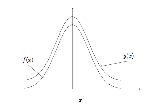
Figure A.4: Concept of a Majorizing Function
Figure A.4 illustrates the concept of a majorizing function for \(f(x)\), which simply means a function that is bigger than \(f(x)\) everywhere.
In addition, to being a majorizing function for \(f(x)\), \(g(x)\) must have finite area. In other words,
\[ c = \int\limits_{-\infty}^{+\infty} g(x) dx \]
If \(w(x)\) is defined as \(w(x) = g(x)/c\) then \(w(x)\) will be a probability density function. The acceptance-rejection method starts by obtaining a random variate \(W\) from \(w(x)\). Recall that \(w(x)\) should be chosen with the stipulation that it can be easily sampled, e.g. via the inverse transform method. Let \(U \sim U(0,1)\). The steps of the procedure are as provided in the following algorithm. The sampling of \(U\) and \(W\) continue until \(U \times g(W) \leq f(W)\) and \(W\) is returned. If \(U \times g(W) > f(W)\), then the loop repeats.
2. Generate \(W \sim w(x)\)
3. Generate \(U \sim U(0,1)\)
4. UNTIL \((U \times g(W) \leq f(W))\)
5. RETURN \(W\)
The validity of the procedure is based on deriving the cumulative distribution function of \(W\) given that the \(W=w\) was accepted, \(P\left\{W \leq x \vert W = w \; \text{is accepted}\right\}\).
The efficiency of the acceptance-rejection method is enhanced as the probability of rejection is reduced. This probability depends directly on the choice of the majorizing function \(g(x)\). The acceptance-rejection method has a nice intuitive geometric connotation, which is best illustrated with an example.
Example A.8 (Acceptance-Rejection Example) Consider the following PDF over the range \(\left[-1,1\right]\). Develop an acceptance/rejection based algorithm for \(f(x)\).
\[ f(x) = \begin{cases} \frac{3}{4}\left( 1 - x^2 \right) & -1 \leq x \leq 1\\ 0 & \text{otherwise}\\ \end{cases} \]
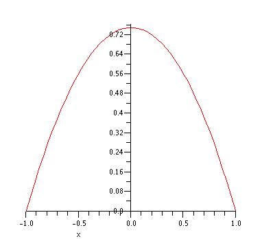
Figure A.5: Plot of f(x)
Solution for Example A.8 The first step in deriving an acceptance/rejection algorithm for the \(f(x)\) in Example A.8 is to select an appropriate majorizing function. A simple method to choose a majorizing function is to set \(g(x)\) equal to the maximum value of \(f(x)\). As can be seen from the plot of \(f(x)\) the maximum value of 3/4 occurs at \(x\) equal to \(0\). Thus, we can set \(g(x) = 3/4\). In order to proceed, we need to construct the PDF associated with \(g(x)\). Define \(w(x) = g(x)/c\) as the PDF. To determine \(c\), we need to determine the area under the majorizing function:
\[ c = \int\limits_{-1}^{1} g(x) dx = \int\limits_{-1}^{1} \frac{3}{4} dx = \frac{3}{2} \]
Thus,
\[ w(x) = \begin{cases} \frac{1}{2} & -1 \leq x \leq 1\\ 0 & \text{otherwise}\\ \end{cases} \]
This implies that \(w(x)\) is a uniform distribution over the range from \(\left[-1,1\right]\). Based on the discussion of the continuous uniform distribution, a uniform distribution over the range from \(a\) to \(b\) can be generated with \(a + U(b-a)\). Thus, for this case (\(a= -1\) and \(b=1\)), with \(b-a = 1 - -1 = 2\). The acceptance rejection algorithm is as follows:
1.1 Generate \(U_{1} \sim U(0,1)\)
1.2 \(W = -1 + 2U_{1}\)
1.3 Generate \(U_{2} \sim U(0,1)\)
1.4 \(f = \frac{3}{4}(1-W^2)\)
2. Until \((U_{2} \times \frac{3}{4} \leq f)\)
3. Return \(W\)
Steps 1.1 and 1.2 of generate a random variate, \(W\), from \(w(x)\). Note that \(W\) is in the range \(\left[-1,1\right]\) (the same as the range of \(X\)) so that step 1.4 is simply finding the height associated with \(W\) in terms of \(f\). Step 1.3 generates \(U_{2}\). What is the range of \(U_{2} \times \frac{3}{4}\)? The range is \(\left[0,\frac{3}{4}\right]\). Note that this range corresponds to the range of possible values for \(f\). Thus, in step 2, a point between \(\left[0,\frac{3}{4}\right]\) is being compared to the candidate point’s height \(f(W)\) along the vertical axis. If the point is under \(f(W)\), the \(W\) is accepted; otherwise the \(W\) is rejected and another candidate point must be generated. In other words, if a point “under the curve” is generated it will be accepted.
As illustrated in the previous, the probability of acceptance is related to how close \(g(x)\) is to \(f(x)\). The ratio of the area under \(f(x)\) to the area under \(g(x)\) is the probability of accepting. Since the area under \(f(x)\) is 1, the probability of acceptance, \(P_{a}\), is:
\[ P_{a} = \frac{1}{\int\limits_{-\infty}^{+\infty} g(x) dx} = \frac{1}{c} \]
where \(c\) is the area under the majorizing function. For the example, the probability of acceptance is \(P_{a} = 2/3\). Based on this example, it should be clear that the more \(g(x)\) is similar to the PDF \(f(x)\) the better (higher) the probability of acceptance. The key to efficiently generating random variates using the acceptance-rejection method is finding a suitable majorizing function over the same range as \(f(x)\). In the example, this was easy because \(f(x)\) had a finite range. It is more challenging to derive an acceptance rejection algorithm for a probability density function, \(f(x)\), if it has an infinite range because it may be more challenging to find a good majorizing function.
A.2.4 Mixture Distributions, Truncated Distributions, and Shifted Random Variables
This section describes three random variate generation methods that build on the previously discussed methods. These methods allow for more flexibility in modeling the underlying randomness. First, let’s consider the definition of a mixture distribution and then consider some examples.
Notice that the \(\omega_{i}\) can be interpreted as a discrete probability distribution as follows. Let \(I\) be a random variable with range \(I \in \left\{ 1, \ldots, k \right\}\) where \(P\left\{I=i\right\} = \omega_{i}\) is the probability that the \(i^{th}\) distribution \(F_{X_{i}}(x)\) is selected. Then, the procedure for generating from \(F_{X}(x)\) is to randomly generate \(I\) from \(g(i) = P\left\{I=i\right\} = \omega_{i}\) and then generate \(X\) from \(F_{X_{I}}(x)\). The following algorithm presents this procedure.
2. Generate \(X \sim F_{X_{I}}(x)\)
3. return \(X\)
Because mixture distributions combine the characteristics of two or more distributions, they provide for more flexibility in modeling. For example, many of the standard distributions that are presented in introductory probability courses, such as the normal, Weibull, lognormal, etc., have a single mode. Mixture distributions are often utilized for the modeling of data sets that have more than one mode.
As an example of a mixture distribution, we will discuss the hyper-exponential distribution. The hyper-exponential is useful in modeling situations that have a high degree of variability. The coefficient of variation is defined as the ratio of the standard deviation to the expected value for a random variable \(X\). The coefficient of variation is defined as \(c_{v} = \sigma/\mu\), where \(\sigma = \sqrt{Var\left[X \right]}\) and \(\mu = E\left[X\right]\). For the hyper-exponential distribution \(c_{v} > 1\). The hyper-exponential distribution is commonly used to model service times that have different (and mutually exclusive) phases. An example of this situation is paying with a credit card or cash at a checkout register. The following example illustrates how to generate from a hyper-exponential distribution.
Example A.9 (Hyper-Exponential Random Variate) Suppose the time that it takes to pay with a credit card, \(X_{1}\), is exponentially distributed with a mean of \(1.5\) minutes and the time that it takes to pay with cash, \(X_{2}\), is exponentially distributed with a mean of \(1.1\) minutes. In addition, suppose that the chance that a person pays with credit is 70%. Then, the overall distribution representing the payment service time, \(X\), has an hyper-exponential distribution with parameters \(\omega_{1} = 0.7\), \(\omega_{2} = 0.3\), \(\lambda_{1} = 1/1.5\), and \(\lambda_{2} = 1/1.1\).
\[ \begin{split} F_{X}(x) & = \omega_{1}F_{X_{1}}(x) + \omega_{2}F_{X_{2}}(x)\\ F_{X_{1}}(x) & = 1 - \exp \left( -\lambda_{1} x \right) \\ F_{X_{2}}(x) & = 1 - \exp \left( -\lambda_{2} x \right) \end{split} \] Derive an algorithm for this distribution. Assume that you have two pseudo-random numbers, \(u_1 = 0.54\) and \(u_2 = 0.12\), generate a random variate from \(F_{X}(x)\).Solution for Example A.9 In order to generate a payment service time, \(X\), we can use the mixture distribution algorithm.
2. Generate \(v \sim U(0,1)\)
3. If \((u \leq 0.7)\)
4. \(X = F^{-1}_{X_{1}}(v) = -1.5\ln \left(1-v \right)\)
5. else
6. \(X = F^{-1}_{X_{2}}(v) = -1.1\ln \left(1-v \right)\)
7. end if
8. return \(X\)
Using \(u_1 = 0.54\), because \(0.54 \leq 0.7\), we have that
\[ X = F^{-1}_{X_{1}}(0.12) = -1.5\ln \left(1- 0.12 \right) = 0.19175 \]
In the previous example, generating \(X\) from \(F_{X_{i}}(x)\) utilizes the inverse transform method for generating from the two exponential distribution functions. In general, \(F_{X_{i}}(x)\) for a general mixture distribution might be any distribution. For example, we might have a mixture of a Gamma and a Lognormal distribution. To generate from the individual \(F_{X_{i}}(x)\) one would use the most appropriate generation technique for that distribution. For example, \(F_{X_{1}}(x)\) might use inverse transform, \(F_{X_{2}}(x)\) might use acceptance/rejection, \(F_{X_{3}}(x)\) might use convolution, etc. This provides great flexibility in modeling and in generation.
In general, we may have situations where we need to control the domain over which the random variates are generated. For example, when we are modeling situations that involve time (as is often the case within simulation), we need to ensure that we do not generate negative values. Or, for example, it may be physically impossible to perform a task in a time that is shorter than a particular value. The next two generation techniques assist with modeling these situations.
A truncated distribution is a distribution derived from another distribution for which the range of the random variable is restricted. Truncated distributions can be either discrete or continuous. The presentation here illustrates the continuous case. Suppose we have a random variable, \(X\) with PDF, \(f(x)\) and CDF \(F(x)\). Suppose that we want to constrain \(f(x)\) over interval \([a, b]\), where \(a<b\) and the interval \([a, b]\) is a subset of the original support of \(f(x)\). Note that it is possible that \(a = -\infty\) or \(b = +\infty\). Constraining \(f(x)\) in this manner will result in a new random variable, \(X \vert a \leq X \leq b\). That is, the random variable \(X\) given that \(X\) is contained in \([a, b]\). Random variables have a probability distribution. The question is what is the probability distribution of this new random variable and how can we generate from it.
This new random variable is governed by the conditional distribution of \(X\) given that \(a \leq X \leq b\) and has the following form:
\[ f(x \vert a \leq X \leq b) = f^{*}(x) = \begin{cases} \frac{g(x)}{F(b) - F(a)} & a \leq x \leq b\\ 0 & \text{otherwise}\\ \end{cases} \]
where
\[ g(x) = \begin{cases} f(x) & a \leq x \leq b\\ 0 & \text{otherwise}\\ \end{cases} \]
Note that \(g(x)\) is not a probability density. To convert it to a density, we need to find its area and divide by its area. The area of \(g(x)\) is:
\[ \begin{split} \int\limits_{-\infty}^{+\infty} g(x) dx & = \int\limits_{-\infty}^{a} g(x) dx + \int\limits_{a}^{b} g(x) dx + \int\limits_{b}^{+\infty} g(x) dx \\ & = \int\limits_{-\infty}^{a} 0 dx + \int\limits_{a}^{b} f(x) dx + \int\limits_{b}^{+\infty} 0) dx \\ & = \int\limits_{a}^{b} f(x) dx = F(b) - F(a) \end{split} \]
Thus, \(f^{*}(x)\) is simply a “re-weighting” of \(f(x)\). The CDF of \(f^{*}(x)\) is:
\[ F^{*}(x) = \begin{cases} 0 & \text{if} \; x < a \\ \frac{F(x) - F(a)}{F(b) - F(a)} & a \leq x \leq b\\ 0 & \text{if} \; b < x\\ \end{cases} \]
This leads to a straight forward algorithm for generating from \(f^{*}(x)\) as follows:
2. \(W = F(a) + (F(b) - F(a))u\)
3. \(X = F^{-1}(W)\)
4. return \(X\)
Lines 1 and 2 of the algorithm generate a random variable \(W\) that is uniformly distributed on \((F(a), F(b))\). Then, that value is used within the original distribution’s inverse CDF function, to generate a \(X\) given that \(a \leq X \leq b\). Let’s look at an example.
Solution for Example A.10 The CDF of the exponential distribution with mean 10 is:
\[ F(x) = 1 - e^{-x/10} \]
Therefore \(F(3) = 1- \exp(-3/10) = 0.259\) and \(F(6) = 0.451\). The exponential distribution has inverse cumulative distribution function:
\[ F^{-1}(u) = \frac{-1}{\lambda}\ln \left(1-u \right) \]
First, we generate a random number uniformly distributed between \(F(3)\) and \(F(6)\) using \(u = 0.23\):
\[ W = 0.259 + (0.451 - 0.259)\times 0.23 = 0.3032 \]
Therefore, in order to generate the distance we have:
\[ X = -10 \times \ln \left(1 - 0.3032 \right) = 3.612 \]
Lastly, we discuss shifted distributions. Suppose \(X\) has a given distribution \(f(x)\), then the distribution of \(X + \delta\) is termed the shifted distribution and is specified by \(g(x)=f(x - \delta)\). It is easy to generate from a shifted distribution, simply generate \(X\) according to \(F(x)\) and then add \(\delta\).
Solution for Example A.11 The Weibull distribution has a closed form cumulative distribution function:
\[ F(x) = 1- e^{-(x/\beta)^\alpha} \]
Thus, the inverse CDF function is:
\[ F^{-1}(u) = \beta\left[ -\ln (1-u)\right]^{1/\alpha} \]
Therefore to generate the setup time we have:
\[ 5.5 + 5\left[ -\ln (1-0.73)\right]^{1/3} = 5.5+ 5.47= 10.97 \] Within this section, we illustrated the four primary methods for generating random variates 1) inverse transform, 2) convolution, 3) acceptance/rejection, and 4) mixture and truncated distributions. These are only a starting point for the study of random variate generation methods.