4.6 Comparing Two Alternative Configurations for the LOTR Makers
Suppose LOTR Makers is interested in reducing the amount of overtime. They have noticed that a bottleneck forms at the ring making station early in the production release and that the rework station is not sufficiently utilized. Thus, they would like to test the sharing of the rework worker between the two stations. The rework worker should be assigned to both the rework station and the ring making station. If a pair of rings arrives to the ring making station either the master ring maker or the rework worker can make the rings. If both ring makers are available, the master ring maker should be preferred. If a pair of rings needs rework, the rework worker should give priority to the rework. The rework worker is not as skilled as the master ring maker and the time to make the rings varies depending on the maker. The master ring maker still takes a UNIF(5,15) minutes to make rings; however, the shared rework worker has a much more variable process time. The rework worker can make rings in 30 minutes according to an exponential distribution. In addition, the rework worker must walk from station to station to perform the tasks and needs a bit more time to change from one task to the next. It is estimated that it will take the rework work an extra 10 minutes per task. Thus, the rework worker’s ring making time is on average 10 + EXPO(30) minutes, and the rework worker’s time to process rework is now 15+WEIB(15,3) minutes.
In addition to the sharing of the rework craftsman, management has noted that the release of the jobs at the beginning of the day is not well represented by the previous model. In fact, after the jobs are released the jobs go through an additional step before reaching the ring making station. After being released all the paperwork and raw materials for the job are found and must travel to the ring station for the making of the rings. The process takes 12 minutes on average according to an exponential distribution for each pair of rings. There are always sufficient workers available to move the rings to the ring station at the beginning of the day. LOTR Makers Inc. would like an analysis of the time to complete the orders for each of the following systems:
Configuration 1: The system with ring preparation/travel delay with no sharing of the rework craftsman.
Configuration 2: The system with ring preparation/travel delay and the sharing of the rework craftsman.
Figure 4.80 illustrates the two system configurations in the form of activity diagrams. Configuration two illustrates that the two resources (master craftsman and rework craftsman) are shared at the make ring activity by placing the two resources in a larger oval. This oval represents the fact that these two resources are in a set. Notice how the SEIZE and RELEASE arrows from the make ring activity go to the boundary of the oval. This indicates that the make ring activity pulls resources from this set of resources.
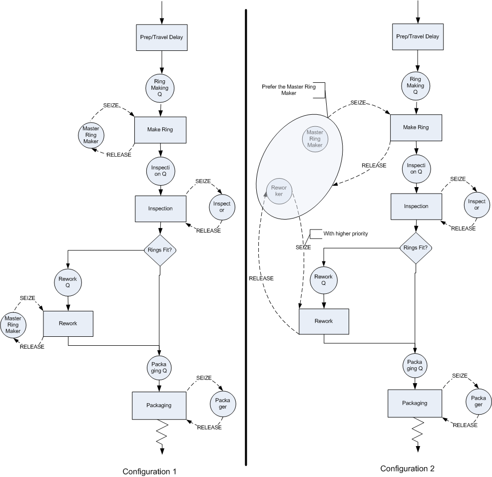
Figure 4.80: Two LOTR alternative configurations
The rework activity still uses the rework craftsman. In particular, the SEIZE and RELEASE arrows go directly to the rework craftsman. The SEIZE arrows have been augmented to indicate that the master craftsman is to be preferred and that the rework activity has higher priority for the rework craftsman. In both activity diagrams the preparation/travel time has been represented with an activity that does not use any resources. This can be modeled with a DELAY module. The implementation of configuration 1 poses no additional modeling challenges; however, for configuration 2, the resource sharing must be modeled.
4.6.1 Resource Sets
The diagram indicates that the master craftsman and the rework craftsman are within the same set. has the capability of defining sets to hold various object types (e.g. resources, queues, etc.). Thus, the set construct can be used to model the sharing of the resources. The set construct is simply a named list of objects of the same type. Thus, a resource set is a list of resources. Each resource listed in the set is called a member of the set. Unlike the mathematical set concept, these sets are ordered lists. Each member of the set is associated with an index representing its order in the list. The first member has an index of 1, the 2nd has an index of 2, and so forth. If you know the index, you can look up which member of the set is associated with the index. In this sense, a set is like an array of objects found in other programming languages. The following illustrates the resource set concept to hold the ring makers.
| Index | Member |
|---|---|
| 1 | RingMakerR |
| 2 | ReworkR |
A set named, RingMakers, can be defined with the two previously
defined resources as members of the set. In this case, the resource
representing the master craftsman (RingMakerR) is placed first in the
set and the resource representing the rework craftsman (ReworkR) is
placed second in the set. The name of the set can be used to return the
associated object:
RingMakers(1)will return the resourceRingMakerRRingMakers(2)will return the resourceReworkR
There are three useful functions for working with sets:
- MEMBER(Set ID, Index)
The
MEMBERfunction returns the construct number of a particular set member. Set ID identifies the set to be examined and index is the index into the set. Using the name of the set with the index number is functionally equivalent to theMEMBERfunction.- MEMIDX(Set ID, Member ID)
The
MEMIDXfunction returns the index value of a construct within the specifiedSet ID.Member IDis the name of the construct.- NUMMEM(Set ID)
The
NUMMEMfunction returns the number of members in the specifiedSet ID.
The ordering of the members in the set may be important to the modeling because of how the rules for selecting members from the set are defined. When an entity attempts to seize a member of the resource set, a resource selection rule may be invoked. The rule will be invoked if there is more than one resource idle at the time that the entity attempts to seize a member of the resource set. There are 7 default rules and 2 ways to specify user defined rules:
- CYC
Selects the first available resource beginning with the successor of the last resource selected. This has the effect of cycling through the resources. For example, if there are 5 members in the set 1,2,3,4,5 and 3 was the last resource selected then 4 will be the next resource selected if it is available.
- POR
Selects the first resource for which the required resource units are available. Each member of the set is checked in the order listed. The order of the list specifies the preferred order of selection.
- LNB
Selects the resource that has the largest number of resource units busy, any ties are broken using the POR rule.
- LRC
Selects the resource that has the largest remaining resource capacity, any ties are broken using the POR rule.
- SNB
Selects the resource that has the smallest number of resource units busy, any ties are broken using the POR rule.
- SRC
Select the resource that has the smallest remaining resource capacity, any ties are broken using the POR rule.
- RAN
Selects randomly from the resources of the set for which the required resource units are available.
- ER(User Rule)
Selects the resource based on rule User Rule defined in the experiment frame.
- UR(User Rule)
Selects the UR\(^{th}\) resource where UR is computed in a user-coded rule function.
Since the master ring maker should be preferred if both are available,
the RingMakerR resource should be listed first in the set and the POR
resource selection rule should used. The only other modeling issue that
must be handled is the fact that the rework worker should show priority
for rework jobs.
From the activity diagram, you can see that there will be two SEIZE modules attempting to grab the rework worker. If the rework worker becomes idle, which SEIZE should have preference? According to the problem, the SEIZE related to the rework activity should be given preference. In the module, you can specify a priority level associated with the SEIZE to handle this case. A lower number results in the SEIZE having a higher priority.
Now, you are ready to implement this situation by modifying the file,
LOTRExample.doe. The files related to this section are available in the book support files for this chapter in a folder called, CompartingTwoSystemsCRN. Open up the submodel named, Ring Processing, and
insert a DELAY module at the beginning of the process as shown in
Figure 4.81. The DELAY module can be found on the
Advanced Process panel. Specify an expo(12) distribution for the delay
time. After making this change, you should save the model under the
name, LOTRConfig1.doe, to represent the first system configuration.
You will now edit this model to create the second system configuration.
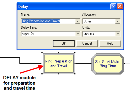
Figure 4.81: DELAY module for preparation and travel time
The first step will be to define the resource set. This can be done using the SET module on the Basic Process panel. Within the SET module, double click on a row to start a new set. Then, you should name the set RingMakers and indicate that the type of set is Resource as shown in Figure 4.82. Now, you can click on the Members area to add rows for each member. Do this as shown in Figure 4.82 and make sure to place RingMakerR and ReworkR as the first and second members in the set. Since the resources had already been defined it is a simple matter of using the drop down textbox to select the proper resources. If you define a set of resources before defining the resources using the RESOURCE module, the programming environment will automatically create the listed resources in the RESOURCE module. You will still have to edit the RESOURCE module.
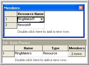
Figure 4.82: Adding members to a resource set
After defining and adding the resources to the set, you should save your
model as LOTRConfig2.doe. You are now ready to specify how to use
the sets within model. Open up the PROCESS module named, Make Ring
Process, in order to edit the previously defined resource specification
for the SEIZE, DELAY, RELEASE logic. In
Figure 4.83, the resource type has been specified as
Set. Then, you should select the RingMakers set using the Preferred Order resource selection rule. You should close up the PROCESS module
and save your model.
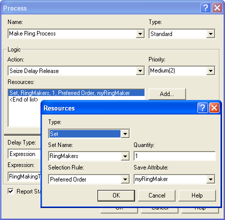
Figure 4.83: Using a resource set in a PROCESS module
Now, you must handle the fact that the processing time to make a ring
depends on which resource is selected. In
Figure 4.83, there is a text field labeled Save
Attribute. This attribute will hold the index number of the resource
that was selected by the SEIZE. In the current situation, this attribute
can be used to have the rings (entity) remember which resource was
selected. This index will have the value 1 or 2 according to whichever
member of the RingMakers set was selected. This index can then be used
to determine the appropriate processing time.
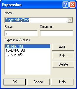
Figure 4.84: Expressions for ring making time by type of worker
Since there are only two ring makers, an arrayed EXPRESSION can be defined, see Figure 4.84, to represent the different processing times. The first expression represents the processing time for the master ring maker and the second expression represents the ring making time of the rework worker. The Save Attribute index can be used to select the appropriate processing time distribution within this arrayed expression. After defining your expressions as shown in Figure 4.84, open up your Make Ring Process module and edit it according to Figure 4.85. Notice how an attribute has been used to remember the index and then that attribute is used to select the appropriate processing time from the EXPRESSION array.
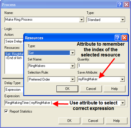
Figure 4.85: Using the save attribute to remember the selected resource and index into the expression
The next required model change is to ensure that the rework craftsman gives priority to rework jobs. This can be done by editing the PROCESS module for the rework process as shown in Figure 4.86. In addition, you need to add an additional 15 minutes for the rework worker’s time to perform the rework due to the job sharing. You are now almost ready to run the models.
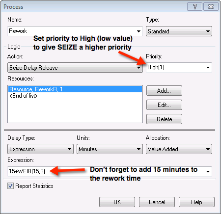
Figure 4.86: Adjusting the priority when seizing the resource
The final change to the model will enable the time to produce the rings to be captured to a file for analysis within the Output Analyzer. Go to the STATISTICS module and add a file name (prodTimeC2.dat) to the OUTPUT statistic for the time to make the order statistics as shown in Figure 4.87. The time to make the orders will be written to the file so that the analysis tools within the Output Analyzer can be used. You should then open up the model file for the first configuration and add an output file (e.g. prodTimeC1.dat) to capture the statistics for the first configuration. You should then run each model for 30 replications.
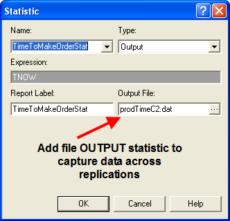
Figure 4.87: Capturing total production time across replication results to a file
After running the models, open up the Output Analyzer and add the two generated files to a new data group. Use the Analyze \(>\) Compare Means option of the Output Analyzer to develop a paired confidence interval for the case of common random numbers. Figure 4.88 illustrates how to set up the Compare Means options. Note that configuration 1 is associated with data file A and configuration 2 is associated with data file B. The default behavior is to compute the difference between A and B (\(\theta = \theta_1 - \theta_2\)). Thus, if \(l > 0\) , you can conclude that configuration 1 has the higher mean time to produce the rings. If this is the case, then configuration 2 would be preferred (shorter production time is better).
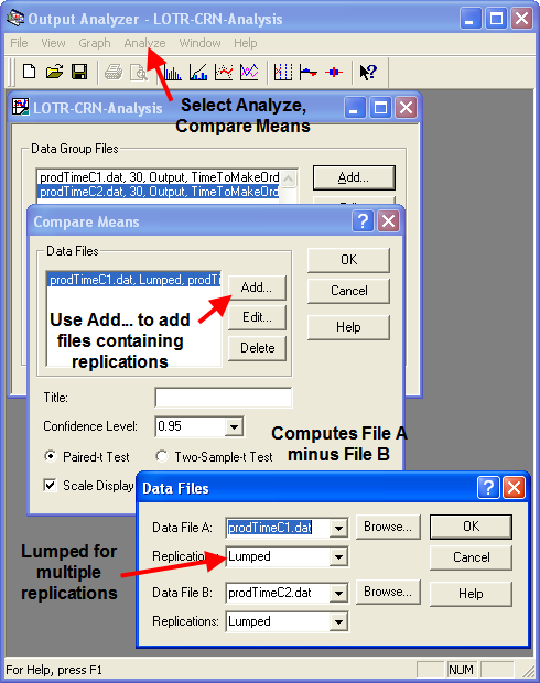
Figure 4.88: Setup paired difference analysis in Output Analyzer
From the results shown in Figure 4.89, you can clearly see that system configuration 2 has the smaller production time. In fact, you can be 95% confident that the true difference between the systems is 92 minutes. This is a practical difference by most standards.
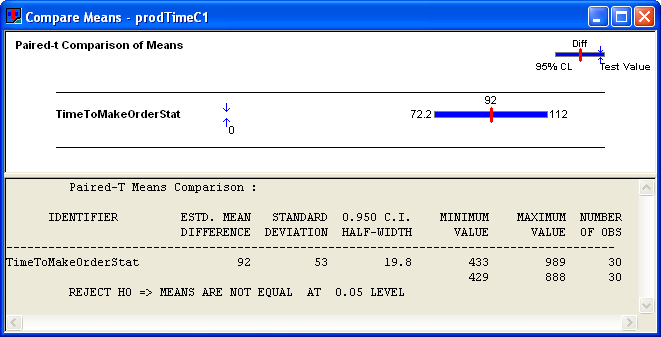
Figure 4.89: Results for the paired difference analysis
Based on these results, LOTR Makers Inc should consider sharing the rework worker between the work stations. If you check the other performance measures as per Figures 4.90 and 4.91, you will see that the utilization of the rework worker is increased significantly (near 97%) in configuration 2.
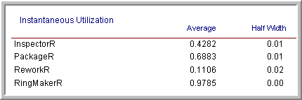
Figure 4.90: Configuration 1 resource utilization
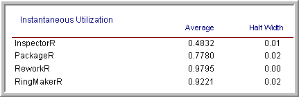
Figure 4.91: Configuration 2 resource utilization
There is also a larger waiting line at the rework station. Such a high utilization for both the ring makers (especially the rework worker) is a bit worrisome. For example, suppose the quality of the work suffered in the new configuration. Then, there would be even more work for the rework worker and possibly a bottleneck at the rework station. Certainly, such a high utilization is troublesome from a human factors standpoint, since worker breaks have not even been modeled! These and other trade-offs can be examined using simulation.
In this example, the performance measure of interest was the time to make the orders. The value of TNOW at the end of the replication represents the time that all of the rings had been produced. This was observed at the end of each replication by using an OUTPUT statistic, as per Figure 4.87. In many situations, we may want to compare performance on measures such as the average system time, the average number of jobs in the system, the resource utilization, etc. In these situations, we need to capture the average of a tally variable or a time-persistent variable at the end of the replication. As noted in Section 3.2, the functions, TAVG(tally ID) and DAVG(dstat ID) will collect the average of the within replication data. Thus, at the end of a replication, these functions hold the average performance of the corresponding tally or time-persistent variable for the current replication. Thus, you can use TAVG(tally ID) and DAVG(dstat ID) in the expression field of the OUTPUT statistic module, as per Figure 4.87, to capture the across replication statistics to a file for post processing using the Output Analyzer. This will be useful in some of the exercises associated with this chapter.
In order to try to ensure a stronger variance reduction when using common random numbers, there are a number of additional implementation techniques that can be applied. For example, to help ensure that the same random numbers are used for the same processes within each of the simulation alternatives you should dedicate a different stream number to each random process in the model. To do this use a different stream number in each probability distribution used within the model. In addition, to help with the synchronization of the use of the random numbers, you can generate the random numbers that each entity will need upon entering the model. Then each entity carries its own random numbers and uses them as it proceeds through the model. In the example, neither technique was done in order to simplify the exposition.
4.6.1.1 Implementing Independent Sampling
This section outlines how to perform the independent sampling case within a model. The completed model files are available as LOTRConfig1IND.doe and LOTRConfig2IND.doe in the folder called ComparingTwoSystemsIND in the book support files for this chapter.
The basic approach to implementing independent sampling is to utilize different random number streams for each configuration. There are a number of different ways to implement the models so that independent sampling can be achieved. The simplest method is to use a variable to represent the stream number in each of the distributions within the model. In LOTRConfig1IND.doe, every distribution was changed as follows:
Sales probability distribution:
BETA(5,1.5, vStream)Success of sale distribution:
DISC(vSalesProb,1,1.0,0, vStream)Preparation and travel time distribution:
EXPO(12,vStream)Master ring make processing time:
UNIF(5,15,vStream)Inner ring diameter:
NORM(vIDM, vIDS, vStream)Outer ring diameter:
NORM(vODM, vODS, vStream)Inspection time distribution:
TRIA(2,4,7,vStream)Rework time distribution:
5+WEIB(15,3, vStream)Packaging time distribution:
LOGN(7,1, vStream)
The same procedure was used for LOTRConfig2IND.doe. Then, the
variable, vStream, was set to different stream numbers so that each
model uses different random number streams. Both models were executed
first using vStream equal to 1 for configuration 1 and vStream equal to
2 for configuration 2. The Output Analyzer can again be used to compare
the results using the Analyze \(>\) Compare Means \(>\) Two sample t-test
option. Figure 4.92 presents the results from the analysis.
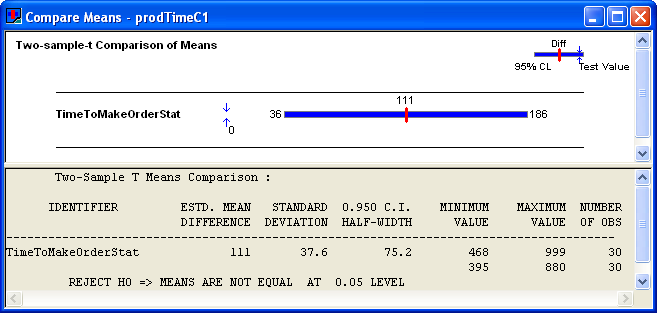
Figure 4.92: Independent two sample analysis from Output Analyzer
The results indicate that configuration 2 has a smaller production time. Notice that the confidence interval for the independent analysis is wider than in the case of common random numbers. This indicates that there is more variability in the independent analysis than in the analysis that used common random numbers.
Since comparing two systems through independent samples takes additional work in preparing the model, one may wonder when it should be applied. If the results from one of the alternatives are already available, but the individual replication values are unavailable to perform the pairing, then the independent sample approach might be used. For example, this might be the case if you were comparing to already published results. In addition, suppose the model takes a very long time to execute and only the summary statistics are available for one of the system configurations. You might want to ensure that the running of the second alternative is independent of the first so that you do not have to re-execute the first alternative. Finally, even though the situation of comparing two simulation runs has been the primary focus of this section, you might have the situation of comparing the results of the simulation to the performance of the actual system. In this case, you can use the data gathered on the actual system and use the two sample independent analysis to compare the results. This is useful in the context of validating the results of the model against the actual system.
This section presented the results for how to compare two alternatives; however, in many situations, you might have many more than two alternatives to analyze. For a small number of alternatives, you might take the approach of making all pair-wise comparisons to develop an ordering. This approach has its limitations which will be discussed in the next section along with how to handle the multiple comparison of alternative.
The last few sections discussed systems that involved queues. In fact, almost all of the models that have been presented within the previous chapters involved queueing lines of some kind. In the next section, we will look at ways to leverage the STATION and ROUTE modules to model more complex networks of queues. This will allow the scaling up of models and facilitate many common modeling situations, found especially in manufacturing environments.