5.7 Exercises
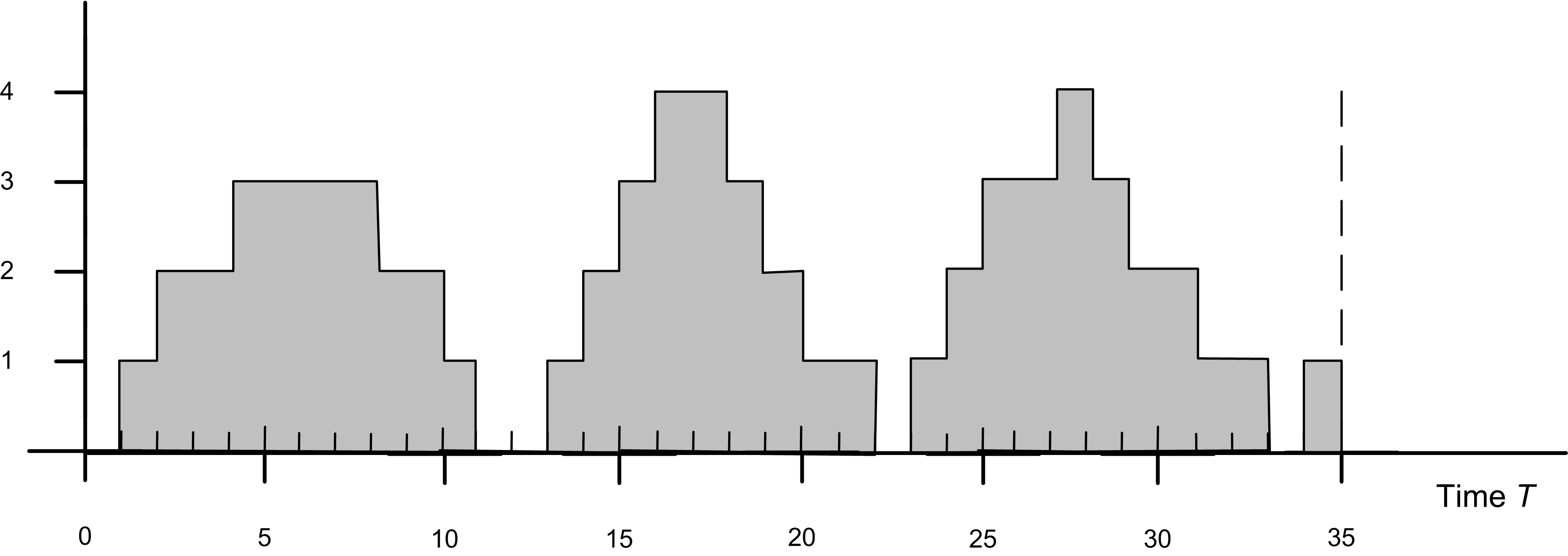
Figure 5.32: Queue length sample path
Exercise 5.6 Using the supplied data set, draw the sample path for the state variable, \(N(t)\). Using a batching interval of 5, apply the batch means method to estimate the average number of customers in the system over the range from 0 to 25. Give a formula for estimating the mean rate of arrivals over the interval from 0 to 25 and then use the data to estimate the mean arrival rate. Estimate the average time in the system (waiting and in service) for the customers indicated in the diagram.
| \(t\) | 0 | 2 | 4 | 5 | 7 | 10 | 12 | 15 | 20 |
| \(N(t)\) | 0 | 1 | 0 | 1 | 2 | 3 | 2 | 1 | 0 |
Develop a 95% confidence interval for your estimate of the mean waiting time based on the data from 1 replication. Discuss why this is inappropriate. How does your simulation estimate compare to the theoretical value?
How does your running average track the theoretical value? What would happen if you increased the number of customers?
Construct a Welch plot using 5 replications of the 1000 customers. Determine a warm up point for this simulation. Do you think that 1000 customers are enough?
Make an autocorrelation plot of your 1000 customer wait times using your favorite statistical analysis package. What are the assumptions for forming the confidence interval in part (a). Is this data independent and identically distributed? What is the implication of your answer for your confidence interval in part (a)?
Use your warm up period from part (c) and generate an addition 1000 customers after the warm up point. Use the method of batch means to batch the 1000 observations into 40 batches of size 25. Make an autocorrelation plot of the 40 batch means. Compute a 95% confidence interval for the mean waiting time using the 40 batches.
Use the method of replication deletion to develop a 95% confidence interval for the mean waiting time. Use your warm period from part (c). Compare the result with that of (a) and (e) and discuss.
Exercise 5.8 YBox video game players arrive at a two-person station for testing. The inspection time per YBox set is EXPO(10) minutes. On the average 82% of the sets pass inspection. The remaining 18% are routed to an adjustment station with a single operator. Adjustment time per YBox is UNIF(7,14) minutes. After adjustments are made, the units are routed back to the inspection station to be retested. Build an simulation model of this system. Use a replication length of 30,000 minutes.
Perform a warm up analysis of the total time a set spends in the system and estimate the system time to within 2 minutes with 95% confidence.
Collect statistics to estimate the average number of times a given job is adjusted.
Suppose that any one job is not allowed more than two adjustments, after which time the job must be discarded. Modify your simulation model and estimate the number of discarded jobs.
Exercise 5.10 A small manufacturing system produces three types of parts. There is a 30% chance of getting a Type 1 part, a 50% chance of getting a Type 2 part and a 20% chance of getting a Type 3 part. The parts arrive from an upstream process such that the time between arrivals is exponentially distributed with a mean of 3 minutes. All parts that enter the system must go through a preparation station where there are 2 preparation workers. The preparation time is exponentially distributed with means 3, 5, and 7 for part types 1, 2, and 3, respectively.
There is only space for 6 parts in the preparation queue. Any parts that that arrive to the system when there are 6 or more parts in the preparation queue cannot enter the system. These parts are shunted to a re-circulating conveyor, which takes 10 minutes to re-circulate the parts before they can try again to enter the preparation queue. Hint: Model the re-circulating conveyor as a simple deterministic delay.
After preparation, the parts are processed on two different production lines. A production line is dedicated to type 1 parts and a production line is dedicated to type 2 and 3 parts. Part types 2 and 3 are built one at a time on their line by 1 of 4 operators assigned to the build station. The time to build a part type 2 or 3 part is triangularly distributed with a (min = 5, mode = 10, max = 15) minutes. After the parts are built they leave the system.
Part type 1 has a more complicated process because of some special tooling that is required during the build process. In addition, the build process is separated into two different operations. Before starting operation 1, the part must have 1 of 10 special tooling fixtures. It takes between 1 and 2 minutes uniformly distributed to place the part in the tooling fixture. An automated machine places the part in the tooling so that the operator at operation 1 does not have to handle the part. There is a single operator at operation 1 which takes 3 minutes on average exponentially distributed. The part remains in the tooling fixture after the first operation and proceeds to the second operation. There is 1 operator at the second operation which takes between 3 and 6 minutes uniformly distributed. After the second operation is complete, the part must be removed from the tooling fixture. An automated machine removes the part from the tooling so that the operator at operation 2 does not have to handle the part. It takes between 20 and 30 seconds uniformly distributed to remove the part from the tooling fixture. After the part is built, it leaves the system.
In this problem, the steady state performance of this system is required in order to identify potential long-term bottlenecks in this process. For this analysis, collect statistics on the following quantities:Queue statistics for all stations. Utilization statistics for all resources.
The system time of parts by part type. The system time should not include the time spent on the re-circulating conveyor.
The average number of parts on the conveyor.
Perform a warm up analysis on the system time of a part regardless of type.
Exercise 5.12 A patient arrives at the Emergency Room about every 20 \(\pm\) 10 minutes (stream 1). The notation X \(\pm\) Y means uniformly distributed with minimum \(X-Y\) and maximum \(X+Y\). They will be treated by either of two doctors.
Twenty percent of the patients are classified as NIA (need immediate attention) and the rest as CW (can wait). NIA patients are given the highest priority, 3, see a doctor as soon as possible for 40 \(\pm\) 37 minutes (stream 2), then have their priority reduced to 2 and wait until a doctor is free again, when they receive further treatment for 30 \(\pm\) 25 minutes (stream 3) and are discharged.
CW patients initially receive a priority of 1 and are treated (when their turn comes) for 15 \(\pm\) 14 minutes (stream 4); their priority is then increased to 2, they wait again until a doctor is free, receive 10 \(\pm\) 8 minutes (stream 5) of final treatment, and are discharged.
An important aspect of this system is that patients that have already seen the doctor once compete with newly arriving patients that need a doctor. As indicated, patients who have already seen the doctor once, have a priority level of 2 (either increased from 1 to 2 or decreased from 3 to 2). Thus, there is one shared queue for the first treatment activity and the final treatment activity. Hint: While there are a number of ways to address this issue you might want to look up Shared Queue in the Help files. In addition, we assume that the doctors are interchangeable. That is, it does not matter which of the 2 doctors performs the first or final treatment. Assume that the initial treatment activity has a higher priority over the final treatment for a doctor.
Simulate for 20 days of continuous operation, 24 hours per day. Precede this by a 2-day initialization period to load the system with patients.
Measure the average queue length of NIA patients from arrival to first seeing a doctor. What percent have to wait to see the doctor for the first treatment? Report statistics on the initial waiting time for NIA patients. What percent wait less than 5 minutes before seeing a doctor for the first time? Report statistics on the time in system for the patients. Report statistics on the remaining time in system from after the first treatment to discharge, for all patients. Discuss what changes to your model are necessary if the doctors are not interchangeable. That is, suppose there are two doctors: Dr. House and Dr. Wilson. The patient must get the same doctor for their final treatment as for their first treatment. For example, if a patient gets Dr. House for their first treatment, they must see Dr. House for their final treatment. You do not have to implement the changes.
Exercise 5.14 An airline ticket office has two ticket agents answering incoming phone calls for flight reservations. In addition, six callers can be put on hold until one of the agents is available to take the call. If all eight phone lines (both agent lines and the hold lines) are busy, a potential customer gets a busy signal, and it is assumed that the call goes to another ticket office and that the business is lost. The calls and attempted calls occur randomly (i.e. according to Poisson process) at a mean rate of 15 per hour. The length of a telephone conversation has an exponential distribution with a mean of 4 minutes.
In addition, the ticket office has instituted an automated caller identification system that automatically places First Class Business (FCB) passengers at the head of the queue, waiting for an agent. Of the original 15 calls per hour, they estimate that roughly one-third of these come from FCB customers. They have also noticed that FCB customers take approximately 3 minutes on average for the phone call, still exponentially distributed. Regular customers still take on average 4 minutes, exponentially distributed. Simulate this system with and without the new prioritization scheme and compare the average waiting time for the two types of customers.Run the simulation for exactly 20000 minutes and estimate for each station the expected average delay in queue for the customer, the expected time-average number of customers in queue, and the expected utilization. In addition, estimate the average number of customers in the system and the average time spent in the system.
Use the results of queueing theory to verify and validate your results for part (a)
Suppose now there is a travel time from the exit of station 1 to the arrival to station 2. Assume that this travel time is distributed uniformly between 0 and 2 minutes. Modify your simulation and rerun it under the same conditions as in part (a).
Exercise 5.17 Parts arrive to a machine shop according to an exponential distribution with a mean of 10 minutes. Before the parts go into the main machining area they must be prepped. The preparation area has two preparation machines that are tended by 2 operators. Upon arrival parts are assigned to either of the two preparation machines with equal probability. Except for processing times the two preparation machines operate in the same manner. When a part enters a preparation machine’s area, it requires the attention of an operator to setup the part on the machine. After the machine is setup, the machine can process without the operator. Upon completion of the processing, the operator is required to remove the part from the machine. The same operator does all the setups and part removals. The operator attends to the parts in a first come, first served manner. The times for the preparation machines are given in the table below according to a triangular distribution with the provided parameters:
| Prep Machine | Setup Time | Process Time | Removal Time |
|---|---|---|---|
| 1 | (8,11,16) | (15,20,23) | (7,9,12) |
| 2 | (6,8,14) | (11,15,20) | (4,6,8) |
After preparation the parts must visit the machine shop. There are 4 machines in the machine shop. The parts follow a specific sequence of machines within the shop. This is determined after they have been prepped. The percentage for each sequence is given in the table below. The #,(min, mode, max) provides the machine number, #, and the parameters for the processing times for a triangular distribution in minutes.
| Sequence | % | #,(min, mode, max) | #,(min, mode, max) | #,(min, mode, max) | #,(min, mode, max) |
|---|---|---|---|---|---|
| 1 | 12 | 1,(10.5,11.9,13.2) | 2, (7.1,8.5,9.8) | 3,(6.7,8,10) | 4, (1,8.9,10.3) |
| 2 | 14 | 1,(7.3,8.6,10.1) | 3,(5.4,7.2, 11.3) | 2,(9.6, 11.4, 15.3) | |
| 3 | 31 | 2,(8.7,9.9,12) | 4,(8.6,10.3,12.8) | 1,(10.3, 12.4, 14.8) | 3,(8.4,9.7,11) |
| 4 | 24 | 3,(7.9,9.3, 10.9) | 4,(7.6,8.9,10.3) | 3,(6.5,8.3,9.7) | 2,(6.7,7.8,9.4) |
| 5 | 19 | 2,(5.6,7.1,8.8) | 1,(8.1, 9.4, 11.7) | 4,(9.1, 10.7, 12.8) |
The transfer time between the prep area and the first machine in the sequence, between all machines, and between the last machine and the system exit follows a triangular distribution with parameters 2, 4, 6 minutes.
Run the model for 200,000 minutes. Report average and 95% half-width statistics on the utilization of the preparation operator, the utilization of the preparation machines, the utilization of the job shop machines 1-4, number of parts in the system, and time spent in the system (in minutes).
Recommend a warm up period for the total time spent in the system. Show your work to justify your recommendation.
Where is the bottleneck for this system? What would you recommend to improve the performance of this system?
Exercise 5.18 Consider the simple three-workstation flow line. Parts entering the system are placed at a staging area for transfer to the first workstation. The staging area can be thought as the place where the parts enter the system prior to going to the first workstation. No processing takes place at the staging area, other than preparation to be directed to the appropriate stations. After the parts have completed processing at the first workstation, they are transferred to a paint station manned by a second worker, and then to a packaging station where they are packed by a third worker, and then to a second staging area where they exit the system.
The time between part arrivals at the system is exponentially distributed with a mean of 28 minutes (stream 1). The processing time at the first workstation is uniformly distributed between 21 and 25 minutes (stream 2). The paint time is log-normally distributed with a mean of 22 minutes and a standard deviation of 4 (stream 3). The packing time follows a triangular distribution with a minimum of 20, mode of 22, and a maximum of 26 (stream 4). The transfers are unconstrained, in that they do not require a vehicle or resource, but all transfer times are exponential with a mean of 2 or 3 minutes (stream 5). Transfer times from the staging to the workstation and from pack to exit are 3 minutes. Transfer times from the workstation to paint and from paint to pack are 2 minutes. The performance measures of interest are the utilization and Work-In-Progress (WIP) at the workstation, paint and packaging operations. Figure 5.33 provides an illustration of the system.
(This problem is based on an example on page 209 and continues on page 217 of (Pegden, Shannon, and Sadowski 1995). Used with permission)
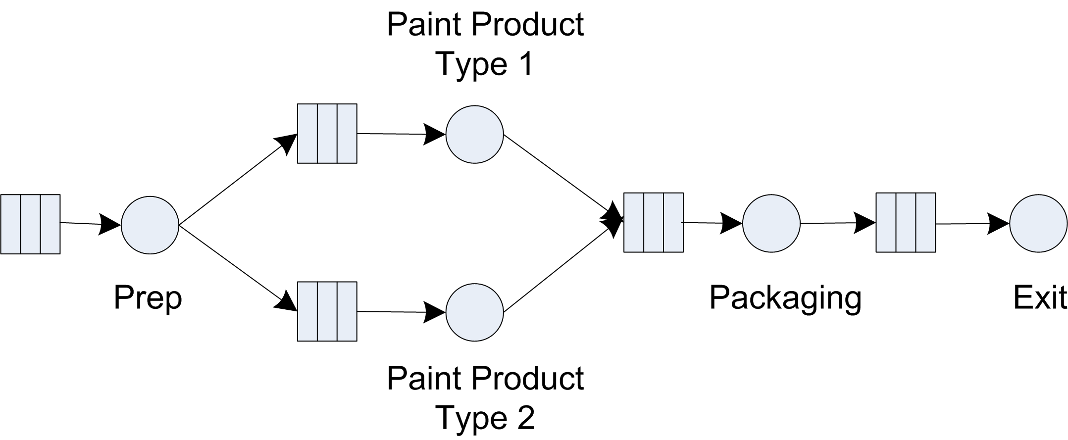
Figure 5.33: Simple painting flow line
Suppose that statistics on the part flow time, i.e. the total time a part spends in the system need to be collected. However, before simulating this process, it is discovered that a new part needs to be considered. This part will be painted a different color. Because the new part replaces a portion of the sales of the first part, the arrival process remains the same, but 30 percent of the arriving parts are randomly designated as the new type of part (stream 10). The remaining parts (70% of the total) are produced in the same manner as described above. However, the new part requires the addition of a different station with a painting time that is log-normally distributed with a mean of 49 minutes and a standard deviation of 7 minutes (stream 6). Assume that an additional worker is available at the new station. The existing station paints only the old type of part and the new station paints only the new parts. After the painting operation, the new part is transferred to the existing packing station and requires a packing time that follows a triangular distribution with a minimum value of 21, a mode of 23, and a maximum of 26 (stream 7). Run the model for 600,000 minutes with a 50,000 minute warm up period. If you were to select a resource to add capacity, which would it be?