8.4 Detailed Modeling
Given your conceptual understanding of the problem, you should now be ready to do more detailed modeling in order to prepare for implementing the model within . When doing detailed modeling it is often useful to segment the problem into components that can be more easily addressed. This is the natural problem solving technique called divide and conquer. Here you must think of the major system components, tasks, or modeling issues that need to be addressed and then work on them first separately and then concurrently in order to have the solution eventually come together as a whole. The key modeling issues for the problem appear to be:
Conveyor and station modeling (i.e. the physical modeling)
Modeling samples
Test Cell modeling including failures
Modeling sample holders
Modeling the load/unload area
Performance measure modeling (cost and statistical collection)
Simulation horizon and run parameters
The following sections will examine each of these issues in turn.
8.4.1 Conveyor and Station Modeling
Recall that conveyor constructs require that each segment of a conveyor be associated with stations within the model. From the problem, the conveyor should be 48 total feet in length. In addition, the problem gives 5 foot and 3 foot distances between the respective enter and exit points. Since the samples access the conveyor 3 feet from the location that they exited the conveyor, a segment is required for this 3 foot distance for the load/unload area and for each of the test cells. Thus, a station will be required for each exit and enter point on the conveyor. Therefore, there are 12 total stations required in the model. The Exit point for the load/unload machine can be arbitrarily selected as the first station on the loop conveyor.
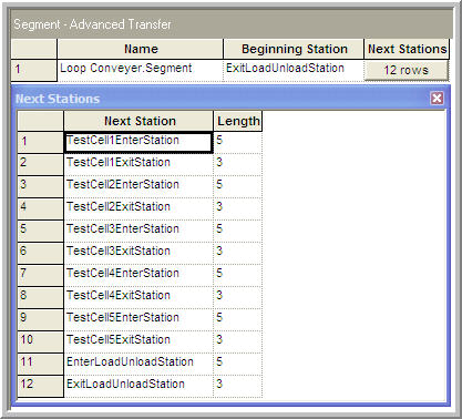
Figure 8.17: Modeling the conveyor segments
Figure 8.17 shows the segments for the conveyor. The test cells as well as the load/unload machine have exit and enter stations that define the segments. The exit point is for exiting the cell to access the conveyor. The enter point is for entering the cell (getting off of the conveyor). Since this is a loop conveyor, the last station listed on the segments should be the same as the first station used to start the segments. The problem also indicates that the sample holder takes up 1 foot when riding on the conveyor. Thus, it seems natural to model the cell size for the conveyor as 1 foot.
The conveyor module for this situation is shown in Figure 8.18. The velocity of the conveyor is 1 foot per second with a cell size of 1 foot. Since a sample holder takes up 1 foot on the conveyor and the cell size is 1 foot, the maximum number of cells occupied by an entity on the conveyor is simply 1 cell.
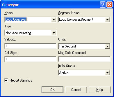
Figure 8.18: Specifying the conveyor module
Since the stations are defined, the sequences within the model can now be defined. How you implement the sequences depends on how the conveyor is modeled and on how the physical locations of the work cells are mapped to the concept of stations. As in any model, there are a number of different methods to achieve the same objective. With stations defined for each entry and exit point, the sequences may use each of the entry and exit points. It should be clear that the entry points must be on the sequences; however, because the exit points are also stations you have the option of using them on the sequences as well. By using the exit point on the sequence, a ROUTE module can be used with the by sequence option to send a sample/sample holder to the appropriate exit station after processing. This could also be achieved by a direct connection, in which case it would be unnecessary to have the exit stations within the sequences. Figure 8.19 illustrates the sequence of stations for test sequence 1 for the problem. Notice that the stations alternate (enter then exit) and that the last station is the station representing the entry point for the load/unload area.
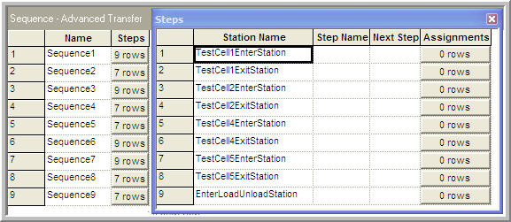
Figure 8.19: Specifying the job steps for test sequence 1
In order to randomly assign a sequence, the sequences can be placed into
a set and then the index into the set randomly generated via the
appropriate probability distribution.
Figure 8.20 shows the Advanced Set module used to
define the set of sequences for the model. In addition,
Figure 8.21 shows the implementation of
the distribution across the sequences as an expression, called
eSeqIndex, using the DISC() function within the EXPRESSION module.
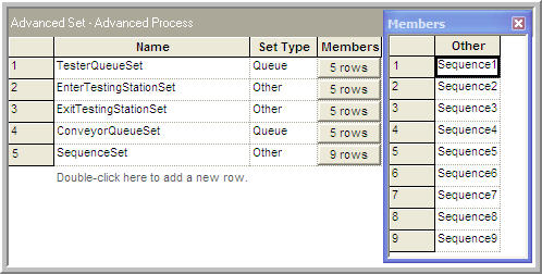
Figure 8.20: Filling the set for holding the sequences
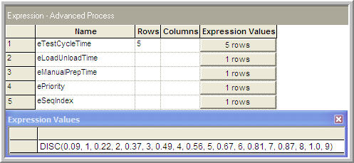
Figure 8.21: Discrete distribution for assigning random sequences
8.4.2 Modeling Samples and the Test Cells
When modeling a large complex problem, you should try to start with a simplified situation. This allows a working model to be developed without unnecessarily complicating the modeling effort. Then, as confidence in the basic model improves, enhancements to the basic model can take place. It will be useful to do just this when addressing the modeling of samples and sample holders.
As indicated in the activity diagrams, once a sample has a sample holder, the sample holder and sample essentially become one entity as they move through the system. Thus, a sample also follows the basic flow as laid out in Figure 8.16. This is essentially what happens to the sample when it is in the black box of Figure 8.15. Thus, to simplify the modeling, it is useful to assume that a sample holder is always available whenever a sample arrives. Since sample holders are not being modeled, there is no need to model the details of the load/unload machine. This assumption implies that once a sample completes its sequence it can simply exit at the load/unload area, and that any newly arriving samples simply get on at the load/unload area. With these assumptions, the modeling of the sample holders and the load/unload stations (including its complicated rules) can be by passed for the time being.
From the conceptual model (activity diagram), it should be clear that the testers can be easily modeled with the RESOURCE module. In addition, the diagram indicates that the logic at any test cell is essentially the same. This could lead to the use of generic stations. Based on all these ideas, you should be able to develop pseudo-code for this situation. If you are following along, you might want to pause and sketch out your own pseudo-code for the simplified modeling situation.
Samples are created according to a non-stationary arrival pattern and then are routed to the exit point for the load/unload station. Then, the samples access the conveyor and are conveyed to the appropriate test cell according to their sequence. Once at a test cell, they test if there is room to get off the conveyor. If so, they exit the conveyor and then use the appropriate tester (SEIZE, DELAY, RELEASE). After using the tester, they are routed to the exit point for the test cell, where they access the conveyor and are conveyed to the next appropriate station. If space is not available at the test cell, they do not exit the conveyor, but rather are conveyed back to the test cell to try again. Once the sample has completed its sequence, the sample will be conveyed to the enter load/unload area, where it exits the conveyor and is disposed. The following pseudo-code illustrates these concepts.
CREATE sample according to non-stationary pattern
BEGIN ASSIGN
    myEnterSystemTime = TNOW
    myPriorityType ~ Priority CDF
END ASSIGN
DELAY  for manual preparation time
ROUTE  to ExitLoadUnloadStation

STATION ExitLoadUnLoadStation
BEGIN ASSIGN
    mySeqIndex ~ Sequence CDF
    Entity.Sequence = MEMBER(SequenceSet, mySeqIndex)
    Entity.JobStep = 0
END ASSIGN
ACCESS Loop Conveyor
CONVEY by Sequence

STATION Generic Testing Cell Enter
DECIDE
    IF NQ at testing cell < cell waiting capacity
        EXIT Loop Conveyor
        SEIZE 1 unit of tester
        DELAY for testing time
        RELEASE 1 unit of tester
        ROUTE to Generic Testing Cell Exit
    ELSE
        CONVEY back to Generic Testing Cell Enter
    ENDIF
END DECIDE

STATION Generic Testing Cell Exit
ACCESS Loop Conveyor
CONVEY by Sequence

STATION EnterLoadUnloadStation
EXIT Loop Conveyor
RECORD System time
DISPOSE
Given the pseudo-code and the previous modeling, you should be able to develop an initial model for this simplified situation. For practice, you might try to implement the ideas that have been discussed before proceeding.
The model (with animation) representing this initial modeling is given in the file, SMTestingInitialModeling.doe. The flow chart modules corresponding to the pseudo-code are shown in Figure 8.22.
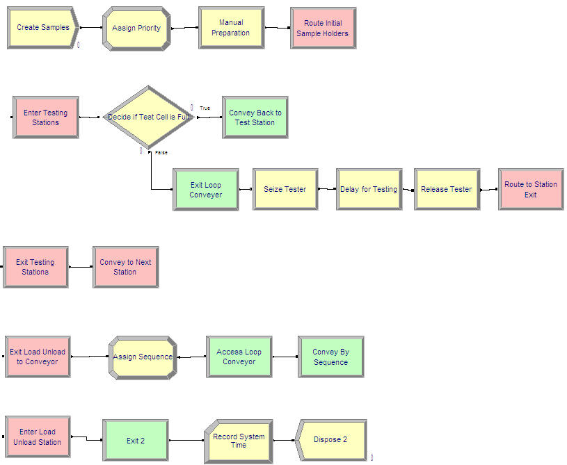
Figure 8.22: Initial model for samples and test cells
The following approach was taken when developing the initial model for samples and test cells:
Variables A variable array,
vTestCellCapacity(5), was defined to hold the capacity of each test cell. While for this particular problem, the cell capacity was the same for each cell, by making a variable array, the cell capacity can be easily varied if needed when testing the various design configurations.Expressions An arrayed expression,
eTestCycleTime(5), was defined to hold the cycle times for the testing machines. By making these expressions, they can be easily changed from one location in the model. In addition, expressions were defined for the manual preparation time (eManualPrepTime), the priority distribution (ePriority), and the sequence distribution (eSeqIndex).Resources Five separate resources were defined to represent the testers (
Cell1Tester,Cell2Tester,Cell3Tester,Cell4Tester,Cell5Tester)Sets A resource set,
TestCellResourceSet, was defined to hold the test cell resources for use in generic modeling. An entity picture set (SamplePictSet) with 9 members was defined to be able to change the picture of the sample according to the sequence it was following. A queue set,TesterQueueSet, was defined to hold the queues in front of each tester for use in generic modeling. In addition, a queue set,ConveyorQueueSet, was defined to hold the access queue for the conveyor at each test cell. Two station sets were defined to hold the enter (EnterTestingStationSet) and the exit (ExitTestingStationSet) stations for generic station modeling. Finally, a sequence set, SequenceSet, was use to hold the 9 sequences followed by the samples.Schedules An ARRIVAL schedule (see Figure 8.23) was defined to hold the arrival rates by hour to represent the non-stationary arrival pattern for the samples.
Failures Five failure modules were use to model the failure and cleaning associated with the test cells. Four failure modules (Tester 1 Failure, Tester 3 Failure, Tester 4 Failure, and Tester 5 Failure) defined time-based failures and the appropriate repair times. A count based failure was use to model Tester 2’s cleaning after 300 uses. The failures are illustrated in Figure 8.24. An important assumption with the use of the FAILURE module is that the entire resource becomes failed when a failure occurs. It is not clear from the contest problem specification what would happen at a test cell that has more than one tester when a failure occurs. Thus, for the sake of simplicity it will be useful to assume that each unit of a multiple unit tester does not fail individually.
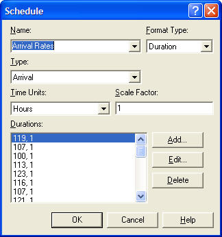
Figure 8.23: ARRIVAL schedule for samples
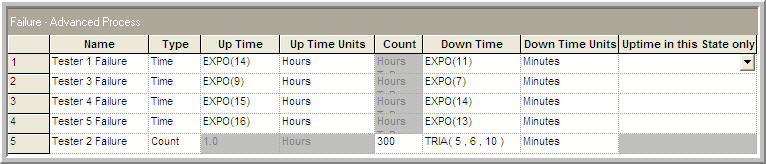
Figure 8.24: FAILURE modules for testers
As a first step towards verifying that the model is working as intended, the initial model, SMTestingInitialModeling.doe, can be modified so that only 1 entity is created. For each of the nine different sequences the total distance traveled on the sequence and the total time for testing can be calculated. For example, for the first sequence, the distance from load/unload exit to the enter location of cell 1 is 5 feet, the distance from cell 1 exit to cell 2 enter is 5 feet, the distance from cell 2 exit to cell 4 enter is 13 feet, the distance from cell 4 exit to cell 5 enter is 5 feet, and finally the distance from cell 5 exit to the enter point for load/unload is 5 feet. This totals 33 feet as shown in Table 8.9. The time to travel 33 feet at 1 foot/second is 0.55 minutes. The total testing time for this sequence is (0.77 + 0.85 +1.24 +1.77 = 5.11) minutes. Finally, the preparation time is 5 minutes for all sequences. Thus, the total time that it should take a sample following sequence 1 should be 10.11 minutes assuming no waiting and no failures. To check that the model can reproduce this quantity, nine different model runs were made such that the single entity followed each of the nine different sequences. The total system time for the single entity was recorded and matched exactly those figures given in Table 8.9. This should give you confidence that the current implementation is working correctly, especially that there are no problems with the sequences. The modified model for testing sequence 9 is given in file, SMTestingInitialModelingTest1Entity.doe.
| Sequence | Steps | Distance | Travel | Test | Preparation | Total |
|---|---|---|---|---|---|---|
| 1 | 1-2-4-5 | 33 | 0.55 | 5.11 | 5 | 10.11 |
| 2 | 3-4-5 | 36 | 0.60 | 3.97 | 5 | 9.57 |
| 3 | 1-2-3-4 | 33 | 0.55 | 3.89 | 5 | 9.44 |
| 4 | 4-3-2 | 132 | 2.20 | 3.12 | 5 | 10.32 |
| 5 | 2-5-1 | 84 | 1.40 | 3.32 | 5 | 9.72 |
| 6 | 4-5-2-3 | 81 | 1.35 | 4.82 | 5 | 11.17 |
| 7 | 1-5-3-4 | 81 | 1.35 | 4.74 | 5 | 11.09 |
| 8 | 5-3-1 | 132 | 2.20 | 3.50 | 5 | 10.70 |
| 9 | 2-4-5 | 36 | 0.60 | 3.79 | 5 | 9.39 |
This testing also provides a lower bound on the expected system times for each of the sequences.
Now that a preliminary working model is available, an initial investigation of the resources required by the system and further verification can be accomplished. From the sequences that are given, the total percentage of the samples that will visit each of the test cells can be tabulated. For example, test cell 1 is visited in sequences 1, 3, 5, 7, and 8. Thus, the total percentage of the arrivals that must visit test cell 1 is (0.09 + 0.15 + 0.07 + 0.14 + 0.06 = 0.51). The total percentage for each of the test cells is given in Table 8.10.
| Cell | 1 | 2 | 3 | 4 | 5 | 6 | 7 | 8 | 9 | Total |
|---|---|---|---|---|---|---|---|---|---|---|
| 1 | 0.09 | 0.00 | 0.15 | 0.00 | 0.07 | 0.00 | 0.14 | 0.06 | 0.00 | 0.51 |
| 2 | 0.09 | 0.00 | 0.15 | 0.12 | 0.07 | 0.11 | 0.00 | 0.00 | 0.13 | 0.67 |
| 3 | 0.00 | 0.13 | 0.15 | 0.12 | 0.00 | 0.07 | 0.11 | 0.13 | 0.00 | 0.71 |
| 4 | 0.09 | 0.13 | 0.15 | 0.12 | 0.00 | 0.00 | 0.11 | 0.14 | 0.13 | 0.87 |
| 5 | 0.09 | 0.13 | 0.00 | 0.00 | 0.07 | 0.11 | 0.14 | 0.06 | 0.13 | 0.73 |
Using the total percentages given in Table 8.10, the mean arrival rate to each of the test cells for each hour of the day can be computed. From the data given in Table 8.6, you can see that the minimum hourly arrival rate is 100 and that it occurs in the 3rd hour. The maximum hourly arrival rate of 200 customers per hour occurs in the \(13^{th}\) hour. From the minimum and maximum hourly arrival rates, you can get an understanding of the range of resource requirements for this system. This will not only help when solving the problem, but will also help in verifying that the model is working as intended.
Let’s look at the peak arrival rate first. From the discussion in Appendix C, the offered load is a dimensionless quantity that gives the average amount of work offered per time unit to the \(c\) servers in a queuing system. The offered load is defined as: \(r = \lambda/\mu\). This can be interpreted as each customer arriving with \(1/\mu\) average units of work to be performed. It can also be thought of as the expected number of busy servers if there are an infinite number of servers. Thus, the offered load can give a good idea of about how many servers might be utilized. Table 8.11 calculates the offered load for each of the test cells under the peak arrival rate.
| Cell | Minutes | Hours | Arrival | Service | Load |
|---|---|---|---|---|---|
| 1 | 0.77 | 0.01283 | 102 | 77.92 | 1.31 |
| 2 | 0.85 | 0.01417 | 134 | 70.59 | 1.90 |
| 3 | 1.03 | 0.01717 | 142 | 58.25 | 2.44 |
| 4 | 1.24 | 0.02067 | 174 | 48.39 | 3.60 |
| 5 | 1.70 | 0.02833 | 146 | 35.29 | 4.14 |
The arrival rate for the first test cell is 0.51 \(\times\) 200 = 102. Thus, you can see that a little over 1 server can be expected to be busy at the first test cell under peak loading conditions.
You can confirm these numbers by modifying the model so that the resource capacities of the test cells are infinite and by removing the failure modules from the resources. In addition, the CREATE module will need to be modified so that the arrival rate is 200 samples per hour. If you run the model for ten, 24 hour days, the results shown in Figure 8.25 will be produced. As can be seen in the figure, the results match very closely to that of the offered load analysis.
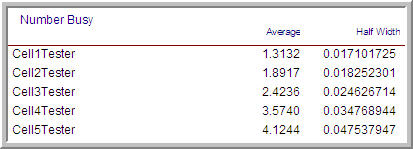
Figure 8.25: Results from offered load experiment
These results provide additional evidence that the initial model is working properly and indicate how many units of each test cell might be needed under peak conditions. The model is given in the file, SMTestingInitialModelingOnResources.doe. Table 8.12 indicates the offered load under the minimum arrival rate.
| Cell | Minutes | Hours | Arrival | Service | Load |
|---|---|---|---|---|---|
| 1 | 0.77 | 0.01283 | 51 | 77.92 | 0.65 |
| 2 | 0.85 | 0.01417 | 67 | 70.59 | 0.95 |
| 3 | 1.03 | 0.01717 | 71 | 58.25 | 1.22 |
| 4 | 1.24 | 0.02067 | 87 | 48.39 | 1.80 |
| 5 | 1.70 | 0.02833 | 73 | 35.29 | 2.07 |
Based on the analysis of the offered load, a preliminary estimate of the resource requirements for each test cell can be determined as in Table 8.13. The requirements were determined by rounding up the computed offered load for each test cell. This provides a range of values since it is not clear that designing to the maximum is necessary given the non-stationary behavior of the arrival of samples.
| Test Cell | Low | High |
|---|---|---|
| 1 | 1 | 2 |
| 2 | 1 | 2 |
| 3 | 2 | 3 |
| 4 | 2 | 4 |
| 5 | 3 | 5 |
8.4.3 Modeling Sample Holders and the Load/Unload Area
Now that a basic working model has been developed and tested, you should feel comfortable with more detailed modeling involving the sample holders and the load/unload area. From the previous discussion, the sample holders appeared to be an excellent candidate for being modeled as an entity. In addition, it also appeared that the sample holders could be modeled as a resource because they also constrain the flow of the sample if a sample holder is not available. There are a number of modeling approaches possible for addressing this situation. By considering the functionality of the load/unload machine, the situation may become more clear. The problem states that:
As long as there are sample holders in front of the load/unload device, it will continue to operate or cycle. It only stops or pauses if there are no available sample holders to process.
Since the load/unload machine is clearly a resource, the fact that sample holders wait in front of it and that it operates on sample holders indicates that sample holders should be entities. Further consideration of the four possible actions of the load/unload machine can provide some insight on how samples and sample holders interact. As a reminder, the four actions are:
The sample holder is empty and the new sample queue is empty. In this case, there is no action required, and the sample holder is sent back to the loop.
The sample holder is empty and a new sample is available. In this case, the new sample is loaded onto the sample holder and sent to the loop.
The sample holder contains a completed sample, and the new sample queue is empty. In this case, the completed sample is unloaded, and the empty sample holder is sent back to the system.
The sample holder contains a completed sample, and a new sample is available. In this case, the completed sample is unloaded, and the new sample is loaded onto the sample holder and sent to the loop.
Thus, if a sample holder contains a sample, it is unloaded during the load/unload cycle. In addition, if a sample is available, it is loaded onto the sample holder during the load/unload cycle. The cycle time for the load/unload machine varies according to a triangular distribution, but it appears as if both the loading and/or the unloading can happen during the cycle time. Thus, whether there is a load, an unload, or both, the time using the load/unload machine is triangularly distributed. If the sample holder has a sample, then during the load/unload cycle, they are separated from each other. If a new sample is waiting, then the sample holder and the new sample are combined together during the processing. This indicates two possible approaches to modeling the interaction between sample holders and samples:
BATCH and SEPARATE The BATCH module can be used to batch the sample and the sample holder together. Then the SEPARATE module can be used to split them apart.
PICKUP and DROPOFF The PICKUP module can be used to have the sample holder pick up a sample, and the DROPOFF module can be used to have the sample holder drop off a completed sample.
Of the two methods, the PICKUP/DROPOFF approach is potentially easier since it puts the sample holder in charge. In the BATCH/SEPARATE approach, it will be necessary to properly coordinate the movement of the sample and the sample holder (perhaps through MATCH, WAIT, SIGNAL modules). In addition, the BATCH module requires careful thought about how to handle the formation of the representative entity and its attributes. In what follows the PICKUP/DROPOFF approach will be used. As an exercise, you might attempt the BATCH/SEPARATE approach.
To begin the modeling of sample holders and samples, you need to think about how they are created and introduced into the model. The samples should continue to be created according to the non-stationary arrival pattern, but after preparation occurs they need to wait until they are picked up by a sample holder. This type of situation can be modeled very effectively with a HOLD module with the infinite hold option specified. In a sense, this is just like the bus system situation of Chapter 7. Now you should be able to sketch out the pseudo-code for this situation.
The pseudo-code for this situation has been developed as shown in the following pseudo-code.
CREATE sample according to non-stationary pattern
BEGIN ASSIGN
    myEnterSystemTime = TNOW
    myPriorityType ~ Priority CDF
END ASSIGN
DELAY for manual preparation time
HOLD until picked up by sample holder

STATION EnterLoadUnloadStation
DECIDE
    IF NQ at load/unload cell >= buffer capacity
        CONVEY back to EnterLoadUnloadStation
    ELSE
        IF sample holder is empty and new sample queue is empty
            CONVEY back to EnterLoadUnloadStation
        ELSE
      EXIT Loop Conveyor
      SEIZE load/unload machine
      DROPOFF sample if loaded
      DELAY for load/unload cycle time
      IF new sample queue is not empty
         PICKUP new sample
      ENDIF
      RELEASE load/unload machine
      ROUTE to ExitLoadUnLoadStation
        ENDIF
    ENDIF
END DECIDE

STATION ExitLoadUnLoadStation
DECIDE
    IF the sample holder has a sample
        BEGIGN ASSIGN
           mySeqIndex ~ Sequence CDF
           Entity.Sequence = MEMBER(SequenceSet, mySeqIndex)
           Entity.JobStep = 0
        END ASSIGN
    ENDIF
END DECIDE
ACCESS Loop Conveyor
DECIDE
    IF the sample holder has a sample
        CONVEY by Sequence
    ELSE
        CONVEY to EnterLoadUnloadStation
    ENDIF
END DECIDE
As seen in the pseudo-code, as a sample holder arrives at the enter point for the load/unload station it first checks to see if there is space in the load/unload buffer. If not, it is simply conveyed back around. If there is space, it checks to see if it is empty and there are no waiting samples. If so, it can simply convey back around the conveyor. Finally, if it is not empty or if there is a sample waiting, it will exit the conveyor to try to use the load/unload machine. If the machine is busy, the sample holder must wait in a queue until the machine is available. Once the machine is seized, it can drop off the sample (if it has one) and pick up a new sample (if one is available). After releasing the load/unload machine, the sample holder possibly with a picked up sample, goes to the exit load/unload station to try to access the conveyor. If it has a sample, it conveys by sequence; otherwise, it conveys back around to the entry point of the load/unload area.
There is one final issue that needs to be addressed concerning the sample holders. How should the sample holders be introduced into the model? As mentioned previously, a CREATE module can be used to create the required number of sample holders at time 0.0. Then, the newly created sample holders can be immediately sent to the ExitLoadUnloadStation. This will cause the newly created and empty sample holders to try to access the conveyor. They will ride around on the conveyor empty until samples start to arrive. At which time, the logic will cause them to exit the conveyor to pick up samples.
Figure 8.26 provides an overview of the entire model. The samples are created, have their priority assigned, experience manual preparation, and then wait in an infinite hold until picked up by the sample holders. The hold queue for the samples is ranked by the priority of the sample, in order to give preference to rush samples. The initial sample holders are created at time 0.0 and routed to the ExitLoadUnloadStation. Two sub-models were used to model the test cells and the load/unload area. The logic for the test cell sub-model is exactly the same as described during the initial model development.
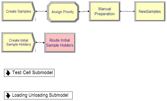
Figure 8.26: Overview of entire model
The file, SMTesting.doe, contains the completed model. The logic described in the previous pseudo-code is implemented in the sub-model, Loading Unloading Submodel. The modeling of the alternate logic is also included in this model.
Now that the basic model is completed, you can concentrate on issues related to running and using the results of the model.
8.4.4 Performance Measure Modeling
Of the modeling issues identified at the beginning of this section, the only remaining issues are the collection of the performance statistics and the simulation run parameters. The key performance statistics are related to the system time and the probability of meeting the contract time requirements. These statistics can be readily captured using RECORD modules. The sub-model for the load/unload area has an additional sub-model that implements the collection of these statistics using RECORD modules. Figure 8.27 illustrates this portion of the model. A variable that keeps track of the number of sample holders in use is decremented each time a sample holder drops off a sample (and incremented any time a sample holder picks up a sample). After the sample is dropped off the number of samples completed is recorded with a counter and the system time is tallied with a RECORD module. The overall probability of meeting the 60 minute limit is tallied using a Boolean expression. Then, the probability is recorded according to whether or not the sample was a rush or not.
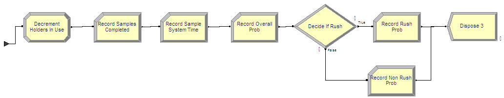
Figure 8.27: System time statistical collection
The cost of each configuration can also be tabulated using output statistics (Figure 8.28). Even though there is no randomness in these cost values, these values can be captured to facilitate the use of the Process Analyzer and OptQuest.
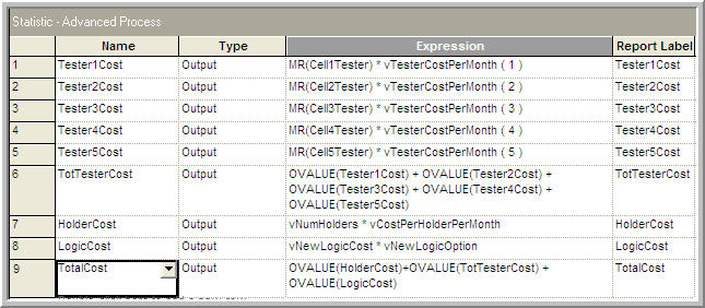
Figure 8.28: STATISTICS module for collecting cost expressions
For example, Table 8.14 shows the total monthly cost calculation for the high resource case assuming the use of 16 sample holders.
| Equipment | Cost per month ($) | # units | Total Cost |
|---|---|---|---|
| Tester Type 1 | 10,000 | 2 | $ 20,000 |
| Tester Type 2 | 12,400 | 2 | $ 24,800 |
| Tester Type 3 | 8,500 | 3 | $ 25,500 |
| Tester Type 4 | 9,800 | 4 | $ 39,200 |
| Tester Type 5 | 11,200 | 5 | $ 56,000 |
| Sample Holder | 387 | 16 | $ 6,192 |
| Total | $ 171,692 |
Now that the model has been set up to collect the appropriate statistically quantities, the simulation time horizon and run parameters must be determined for the experiments.