3.4 Modeling a STEM Career Mixer
In this section, we will model the operation of a STEM Career Fair mixer during a six-hour time period. The purpose of the example is to illustrate the following concepts:
Probabilistic flow of entities using the DECIDE module with the by chance option
Additional options of the PROCESS module
Using the Label module to direct the flow of entities
Collecting statistics on observational (tally) data using the RECORD module
Collecting statistics on time-persistent data using the Statistics panel
Analysis of a finite horizon model to ensure a pre-specified half-width requirement
Example 3.4 Students arrive to a STEM career mixer event according to a Poisson process at a rate of 0.5 student per minute. The students first go to the name tag station, where it takes between 10 and 45 seconds uniformly distributed to write their name and affix the tag to themselves. We assume that there is plenty of space at the tag station, as well has plenty of tags and markers, such that a queue never forms.
After getting a name tag, 50% of the students wander aimlessly around, chatting and laughing with their friends until they get tired of wandering. The time for aimless students to wander around is triangularly distributed with a minimum of 10 minutes, a most likely value of 15 minutes, and a maximum value of 45 minutes. After wandering aimlessly, 90% decide to buckle down and visit companies and the remaining 10% just are too tired or timid and just leave. Those that decide to buckle down visit the MalWart station and then the JHBunt station as described next.
The remaining 50% of the original, newly arriving students (call them non-aimless students), first visit the MalWart company station where there are 2 recruiters taking resumes and chatting with applicants. At the MalWart station, the student waits in a single line (first come first served) for 1 of the 2 recruiters. After getting 1 of the 2 recruiters, the student and recruiter chat about the opportunities at MalWart. The time that the student and recruiter interact is exponentially distributed with a mean of 3 minutes. After visiting the MalWart station, the student moves to the JHBunt company station, which is staffed by 3 recruiters. Again, the students form a single line and pick the next available recruiter. The time that the student and recruiter interact at the JHBunt station is also exponentially distribution, but with a mean of 6 minutes. After visiting the JHBunt station, the student departs the mixer.The organizer of the mixer is interested in collecting statistics on the following quantities within the model:
number of students attending the mixer at any time t
number of students wandering at any time t
utilization of the recruiters at the MalWart station
utilization of the recruiters at the JHBunt station
number of students waiting at the MalWart station
number of students waiting at the JHBunt station
the waiting time of students waiting at the MalWart station
the waiting time of students waiting at the JHBunt station
total time students spend at the mixer broken down in the following manner
all students regardless of what they do and when they leave
students that wander and then visit recruiters
students that do not wander
The STEM mixer organizer is interested in estimating the average time students spend at the mixer (regardless of what they do) to within plus or minus 1 minute with a 95% confidence level.
3.4.1 Conceptualizing the System
When developing a simulation model, whether you are an experienced analyst or a novice, you should follow a modeling recipe. I recommend developing answers to the following questions:
What is the system?
What are the elements of the system?
What information is known by the system?
What are the required performance measures?
What are the entity types?
What information must be recorded or remembered for each entity instance?
How are entities (entity instances) introduced into the system?
What are the resources that are used by the entity types?
- Which entity types use which resources and how?
What are the process flows? Sketch the process or make an activity flow diagram
Develop pseudo-code for the situation
Implement the model in Arena
We will apply each of these questions to the STEM mixer example. The first set of questions: What is the system? What information is known by the system? are used to understand what should be included in the modeling and what should not be included. In addition, understanding the system to be modeled is essential for validating your simulation model. If you have not clearly defined what you are modeling (i. e. the system), you will have a very difficult time validating your simulation model.
The first thing that I try to do when attempting to understand the system is to draw a picture. A hand drawn picture or sketch of the system to be modeled is useful for a variety of reasons. First, a drawing attempts to put down “on paper” what is in your head. This aids in making the modeling more concrete and it aids in communicating with system stakeholders. In fact, a group stakeholder meeting where the group draws the system on a shared whiteboard helps to identify important system elements to include in the model, fosters a shared understanding, and facilitates model acceptance by the potential end-users and decision makers.
You might be thinking that the system is too complex to sketch or that it is impossible to capture all the elements of the system within a drawing. Well, you are probably correct, but drawing an idealized version of the system helps modelers to understand that you do not have to model reality to get good answers. That is, drawing helps to abstract out the important and essential elements that need to be modeled. In addition, you might think, why not take some photographs of the system instead of drawing? I say, go ahead, and take photographs. I say, find some blueprints or other helpful artifacts that represent the system and its components. These kinds of things can be very helpful if the system or process already exists. However, do not stop at photographs, drawing facilitates free flowing ideas, and it is an active/engaging process. Do not be afraid to draw. The art of abstraction is essential to good modeling practice.
Alright, have I convinced you to make a drawing? So, your next question is, what should my drawing look like and what are the rules for making a drawing? Really? My response to those kinds of questions is that you have not really bought into the benefits of drawing and are looking for reasons to not do it. There are no concrete rules for drawing a picture of the system. I like to suggest that the drawing can be like one of your famous kindergarten pictures you used to share with your grandparents. In fact, if your grandparents could look at the drawing and be able to describe back to you what you will be simulating, you will be on the right track! There are not really any rules.
Well, I will take that back. I have one rule. The drawing should not look like an engineer drew it. Try not to use engineering shapes, geometric shapes, finely drawn arrows, etc. You are not trying to make a blueprint. You are not trying to reproduce the reality of the system by drawing it to perfect scale. You are attempting to conceptualize the system in a form that facilitates communication. Don’t be afraid to put some labels and text on the drawing. Make the drawing a picture that is rich in the elements that are in the system. Also, the drawing does not have to be perfect, and it does not have to be complete. Embrace the fact that you may have to circle back and iterate on the drawing as new modeling issues arise. You have made an excellent drawing if another simulation analyst could take your drawing and write a useful narrative description of what you are modeling.

Figure 3.4: Rich picture system drawing of STEM Career Mixer
Figure 3.4 illustrates a drawing for the STEM mixer problem. As you can see in the drawing, we have students arriving to a room that contains some tables for conversation between attendees. In addition, the two company stations are denoted with the recruiters and the waiting students. We also see the wandering students and the timid students’ paths through the system. At this point, we have a narrative description of the system (via the problem statement) and a useful drawing of the system. We are ready to answer the following questions:
What are the elements of the system?
What information is known by the system?
When answering the question “what are the elements?” your focus should be on two things: 1) the concrete structural things/objects that are required for the system to operate and 2) the things that are operated on by the system (i.e. the things that flow through the system).
What are the elements?
students (non-wanderers, wanderers, timid)
recruiters: 2 for MalWart and 3 for JHBunt
waiting lines: one line for MalWart recruiters, one line for JHBunt recruiters
company stations: MalWart and JHBunt
The paths that students may take.
Notice that the answers to this question are mostly things that we can point at within our picture (or the real system).
When answering the question “what information is known at the system level?” your focus should be identifying facts, input parameters, and environmental parameters. Facts tend to relate to specific elements identified by the previous question. Input parameters are key variables, distributions, etc. that are typically under the control of the analyst and might likely be varied during the use of the model. Environmental parameters are also a kind of input parameter, but they are less likely to be varied by the modeler because they represent the operating environment of the system that is most likely not under control of the analyst to change. However, do not get hung up on the distinction between input parameters and environmental parameters, because their classification may change based on the objectives of the simulation modeling effort. Sometimes innovative solutions come from questioning whether or not an environmental parameter can really be changed.
What information is known at the system level?
students arrive according to a Poisson process with mean rate 0.5 students per minute or equivalently the time between arrivals is exponentially distributed with a mean of 2 minutes
time to affix a name tag ~ UNIF(20, 45) seconds
50% of students are go-getters and 50% are wanderers
time to wander ~ TRIA(10, 15, 45) minutes
10% of wanderers become timid/tired, 90% visit recruiters
number of MalWart recruiters = 2
time spent chatting with MalWart recruiter ~ EXPO(3) minutes
number of JHBunt recruiters = 3
time spent chatting with JHBunt recruiter ~ EXPO(6) minutes
A key characteristic of the answers to this question is that the information is “global.” That is, it is known at the system level. We will need to figure out how to represent the storage of this information when implementing the model within software.
The next question to address is "What are the required performance measures?" For this situation, we have been given as part of the problem a list of possible performance measures, mostly related to time spent in the system and other standard performance measures related to queueing systems. In general, you will not be given the performance measures. Instead, you will need to interact with the stakeholders and potential users of the model to identify the metrics that they need in order to make decisions based on the model. Identifying the metrics is a key step in the modeling effort. If you are building a model of an existing system, then you can start with the metrics that stakeholders typically use to character the operating performance of the system. Typical metrics include cost, waiting time, utilization, work in process, throughput, and probability of meeting design criteria.
Once you have a list of performance measures, it is useful to think about how you would collect those statistics if you were an observer standing within the system. Let’s pretend that we need to collect the total time that a student spends at the career fair and we are standing somewhere at the actual mixer. How would you physically perform this data collection task? In order to record the total time spent by each student, you would need to note when each student arrived and when each student departed. Let \(A_{i}\) be the arrival time of the \(i^{\text{th}}\) student to arrive and let \(D_{i}\) be the departure time of the \(i^{\text{th}}\) student. Then, the system time (T) of the \(i^{\text{th}}\) student is \({T_{i} = D}_{i} - A_{i}\). How could we keep track of \(A_{i}\) for each student? One simple method would be to write the time that the student arrived on a sticky note and stick the note on the student’s back. Hey, this is pretend, right? Then, when the student leaves the mixer, you remove the sticky note from their back and look at your watch to get \(D_{i}\) and thus compute, \(T_{i}\). Easy! We will essentially do just that when implementing the collection of this statistic within the simulation model. Now, consider how you would keep track of the number of students attending the mixer. Again, standing where you can see the entrance and the exit, you would increment a counter every time a student entered and decrement the counter every time a student left. We will essentially do this within the simulation model.
Thus, identifying the performance measures to collect and how you will collect them will answer the 2nd modeling question. You should think about and document how you would do this for every key performance measure. However, you will soon realize that simulation modeling languages, like Arena, have specific constructs that automatically collect common statistical quantities such as resource utilization, queue waiting time, queue size, etc. Therefore, you should concentrate your thinking on those metrics that will not automatically be collected for you by the simulation software environment. In addition to identifying and describing the performance measures to be collected, you should attempt to classify the underlying data needed to compute the statistics as either observation-based (tally) data or time-persistent (time-weighted) data. This classification will be essential in determining the most appropriate constructs to use to capture the statistics within the simulation model. The following table summarizing the type of each performance measure requested for the STEM mixer simulation model.
| Performance Measure | Type |
|---|---|
| Average number of students attending the mixer at any time t | Time persistent |
| Average number of students wandering within the mixer at any time t | Time persistent |
| Average utilization of the recruiters at the MalWart station | Time persistent |
| Average utilization of the recruiters at the MalWart station | Time persistent |
| Average utilization of the recruiters at the JHBunt station | Time persistent |
| Average number of students waiting at the MalWart station | Time persistent |
| Average number of students waiting at the JHBunt station | Time persistent |
| Average waiting time of students waiting at the MalWart station | Tally |
| Average waiting time of students waiting at the JHBunt station | Tally |
| Average system time for students regardless of what they do | Tally |
| Average system time for students that wander and then visit recruiters | Tally |
| Average system time for students that do not wander | Tally |
Now, we are ready to answer the rest of the questions. When performing a process-oriented simulation, it is important to identify the entity types and the characteristics of their instances. An entity type is a classification or indicator that distinguishes between different entity instances. If you are familiar with object-oriented programming, then an entity type is a class, and an entity instance is an object of that class. Thus, an entity type describes the entity instances (entities) that are in its class. An entity instance (or just entity) is something that flows through the processes within the system. Entity instances (or just entities) are realizations of objects within the entity type (class). Different entity types may experience different processes within the system. The next set of questions are about understanding entity types and their instances: What are the entity types? What information must be recorded or remembered for each entity (entity instance) of each entity type? How are entities (entity instances) for each entity type introduced into the system?
Clearly, the students are a type of entity. We could think of having different sub-types of the student entity type. That is, we can conceptualize three types of students (non-wanderers, wanderers, and timid/tired). However, rather than defining three different classes or types of students, we will just characterize one general type of entity called a Student and denote the different types with an attribute that indicates the type of student. An attribute is a named property of an entity type and can have different values for different instances. We will use the attribute, myType, to denote the type of student (1= non-wanders, 2 = wanderers, 3 = timid). Then, we will use this type attribute to help in determining the path that a student takes within the system and when collecting the required statistics.
We are basically told how the students (instances of the student entity type) are introduced to the system. That is, we are told that the arrival process for students is Poisson with a mean rate of 0.5 students per minute. Thus, we have that the time between arrivals is exponential with a mean of 2 minutes. What information do we need to record or be remembered for each student? The answer to this question identifies the attributes of the entity. Recall that an attribute is a named property of an entity type which can take on different values for different entity instances. Based on our conceptualization of how to collect the total time in the system for the students, it should be clear that each entity (student) needs to remember the time that the student arrived. That is our sticky note on their backs. In addition, since we need to collect statistics related to how long the different types of students spend at the STEM fair, we need each student (entity) to remember what type of student they are (non-wanderer, wanderer, and timid/tired). So, we can use the, myType, attribute to note the type of the student.
After identifying the entity types, you should think about identifying the resources. Resources are system elements that entity instances need in order to proceed through the system. The lack of a resource causes an entity to wait (or block) until the resource can be obtained. By the way, if you need help identifying entity types, you should identify the things that are waiting in your system. It should be clear from the picture that students wait in either of two lines for recruiters. Thus, we have two resources: MalWart Recruiters and JHBunt Recruiters. We should also note the capacity of the resources. The capacity of a resource is the total number of units of the resource that may be used. Conceptually, the 2 MalWart recruiters are identical. There is no difference between them (as far as noted in the problem statement). Thus, the capacity of the MalWart recruiter resource is 2 units. Similarly, the JHBunt recruiter resource has a capacity of 3 units.
In order to answer the “and how” part of the question, I like to summarize the entities, resources and activities experienced by the entity types in a table. Recall that an activity is an interval of time bounded by two events. Entities experience activities as they move through the system. The following table summarizes the entity types, the activities, and the resources. This will facilitate the drawing of an activity diagram for the entity types.
| Entity Type | Activity | Resource Used |
|---|---|---|
| Student (all) | time to affix a name tag ~ UNIF(20, 45) seconds | None |
| Student (wanderer) | Wandering time ~ TRIA(10, 15, 45) minutes | None |
| Student (not timid) | Talk with MalWart ~ EXPO(3) minutes | 1 of the 2 MalWart recruiters |
| Student (not timid) | Talk with JHBunt ~ EXPO(6) minutes | 1 of the 3 JHBunt recruiters |
Now we are ready to document the processes experienced by the entities. A good way to do this is through an activity flow diagram. As described in the Chapter 2, an activity diagram will have boxes that show the activities, circles to show the queues and resources, and arrows, to show the paths taken. Figure 3.5 presents the activity diagram for this situation.

Figure 3.5: Activity diagram for STEM Career Mixer
In Figure 3.5, we see that the students are created according to a time between arrival (TBA) process that is exponentially distributed with a mean of 2 minutes and they immediately experience the activity associated with affixing the name tag. Note that the activity does not require any resources and thus has no queue in front of it. Then, the students follow one of two paths, with 50% becoming “non-wanderers” and 50% becoming “wanderers.” The wandering students, wander aimlessly, for period of time, which is represented by another activity that does not require any resources. Then, the 90% of the students follow the non-wanderer path and the remaining 10% of the students, the timid/tired students, leave the system. The students that decide to visit the recruiting stations, first visit the MalWart station, where in the diagram we see that there is an activity box for their talking time with the recruiter. During this talking time, they require one of the recruiters and thus we have a resource circle indicating the usage of the resource. In addition, we have a circle with a queue denoted before the activity to indicate that the students visiting the station may need to wait. The JHBunt station is represented in the same fashion. After visiting the JHBunt station, the students depart the mixer. Now, we are ready to represent this situation using some pseudo-code.
Pseudo-code is simply a computer language like construct for representing the programming elements of a computer program. In this text, we will use pseudo-code that has elements of Arena-like syntax to help document the coding logic, before we use Arena. Let me state that again. Write pseudo-code, before opening up Arena and laying down Arena modules. Why? Pseudo-code facilitates communication of the logic, without a person having to know Arena. Often, other simulation programming environments will have constructs similar to those available within Arena. Thus, your coding logic is more generic. Secondly, pseudo-code is compact and concise. Lastly, having pseudo-code before using Arena has proven over many years to result in better organized models that tend to work correctly.
The following table is an initial listing of pseudo-code syntax that we will utilize within this example. Notice that in the table, I have noted some of the naming conventions that I recommend and some comments about the usage of the construct.
| Keyword | Purpose | Comments |
|---|---|---|
| ATTRIBUTES | To provide a list of attributes and their usage | Attribute names should start with “my” |
| VARIABLES | To provide a list of variables and their usage | Variable names should start with “v” |
| RESOURCES | To provide a list of resources and their capacity | Resource names should start with “r” |
| CREATE | To define a creational pattern | Indicate what is being created and the timing of the creation |
| ASSIGN | To represent the assignment of a value to a variable, attribute, or other construct | BEGIN ASSIGN Multiple assignment statements END ASSIGN |
| DECIDE IF | To represent conditional logic or path choice | DECIDE IF (condition) Executed if condition is true ELSE Executed if condition is false END DECIDE |
| DECIDE with chance | To represent probabilistic path choice | DECIDE with chance: p: Executed with probability p 1-p: Executed with probability 1-p END DECIDE |
| DELAY | To represent a scheduled passage of time for an activity | Indicate the time or distribution associated with the delay and name of activity |
| SEIZE | To represent the need for a resource | Indicate the name of the resource and the number of units required |
| RELEASE | To represent the release of units of a resource | Indicate the name of the resource and the number of units released |
| GOTO: Label | To direct the execution to a particular label | Provide the name of the label |
| Label: Name | To indicate a label where to go | Provide the name of the label |
| RECORD (expression) | To indicate the collection of statistics | BEGIN RECORD Multiple expression statements END RECORD |
| DISPOSE | To represent the disposal of the entity that was executing the code | Implies the release of memory associated with the entity |
These pseudo-code constructs will represent specific modules or programming constructs within the Arena environment. There are a lot more possibilities and variations of these constructs that will be explored throughout the textbook. One such variation is in describing a process. The SEIZE, DELAY, RELEASE combination is so prevalent, you will see that Arena has defined a PROCESS module that provides common variations of usage of these three constructs. Syntactically, we might indicate the usage of a PROCESS module as follows:
BEGIN PROCESS: SEIZE, DELAY, RELEASE
   Resource: worker
   Amount needed: 1
   Delay time: 5 minutes
END PROCESS
This is conceptually the same as writing:
SEIZE 1 worker
DELAY for 5 minutes
RELEASE 1 worker
You decide which you prefer to write. Either case indicates to me that we would use the Arena PROCESS module. I tend to write my pseudo-code in the lowest level of syntax and without worrying about matching perfectly to Arena constructs. The model translation and building phase of the recipe will take care of those worries.
If you have made a rigorous effort to answer the questions and follow the suggested modeling recipe, then the pseudo-code will be a more straightforward exercise than if you did not follow the recipe.
Students often ask, “how do you come up with the pseudo-code so easily?” The answer is that I put in the effort before starting the pseudo-code and I point out that they are seeing the end result. That is, there may be a number of iterations of the pseudo-code before I feel that it is a satisfactory representation of what I will need to build the simulation model. In addition, the pseudo-code does not have to be perfect. You should attempt to capture the essence of what needs to be done and not worry that you have an exact listing for the model building stage.
To start the pseudo-code, it is useful to define some of the structural modeling elements that you will use throughout the code such as the attributes, variables, and resources.
Pseudo-Code Definition Elements

ATTRIBUTES:
myType // represents the type of the student (1= non-wanders, 2 =
wanderers, 3 = timid).
myArrivalTime // the time that the student arrived to the mixer

VARIABLES:
vNumInSys // represents the number of students attending the mixer at
any time t

RESOURCES:
rMalWartRecruiters, 2 // the MalWart recruiters with capacity 2
rJHBuntRecruiters, 3 // the JHBunt recruiters with capacity 3
Considering the pseudo-code for the STEM Fair Mixer example problem, we see the use of ATTRIBUTES, VARIABLES, and RESOURCES to define some elements that will be used throughout the code. Notice the use of “my” and “v” and “r” in the naming of the attributes, variables, and resources.
After defining some of the structural elements needed within the pseudo-code, I then start with introducing the entities into the simulation. That is, I start with the CREATE modules. In addition, I use the activity diagram to assist in determining the logical flow of the pseudo-code and to consider the constructs that will be needed to represent that logical flow.
Pseudo-Code Modeling Elements

CREATE students every EXPO(2) minutes with the first arriving at time
EXPO(2)
BEGIN ASSIGN
   myArrivalTime = TNOW // save the current time in the myArrivalTime attribute
   vNumInSys = vNumInSys + 1
END ASSIGN
DELAY UNIF(15,45) seconds to get name tag
DECIDE with chance:
50%:
   ASSIGN: myType = 1 // non-wandering student
   Goto: Recruiting Stations
50%:
   ASSIGN: myType = 2 // wandering student
   Goto: Wandering
END DECIDE

Label: Wandering
DELAY TRIA(15, 20, 45) minutes for wandering
DECIDE with chance:
10%: Goto: Recruiting Stations
90%:
   ASSIGN: myType = 3 // timid student
   Goto: Exit Mixer
END DECIDE

Label: Recruiting Stations
SEIZE 1 MalWart recruiter
DELAY for EXPO(3) minutes for interaction
RELEASE 1 MalWart recruiter
SEIZE 1 JHBunt recruiter
DELAY for EXPO(6) minutes for interaction
RELEASE 1 JHBunt recruiter
Goto: Exit Mixer

Label: Exit Mixer
ASSIGN: vNumInSys = vNumInSys - 1
ASSIGN: mySysTime = TNOW - myArrivalTime
RECORD mySysTime, as System Time regardless of type
DECIDE IF (myType == 1)
   RECORD mySysTime, as Non-Wandering System Time
ELSE IF (myType ==2)
   RECORD mySysTime, as Wandering System Time
ELSE // myType == 3
   RECORD mySysTime, as Timid Student System Time
END DECIDE
DISPOSE
The modeling code starts off with a CREATE statement that
indicates the Poisson process for the arriving students. Then, we assign
the current simulation clock time, TNOW, to the attribute myArrvalTime.
TNOW is a global, non-user assignable variable that contains the current
simulation time represented in the base time units of the simulation.
After getting marked with their arrival time, we increment the number of
students attending the mixer. Then, the student entity performs the name
tag activity for the designated time. Because there is a 50-50 chance
associated with wandering or not wandering, we use a DECIDE with chance
construct and set the type of the student via the myType attribute
before sending the student on the rest of their path. Notice the use of
labels to denote where to send the entity (student). If the student is a
wanderer, there is a delay to indicate the time spent wandering, and
then another DECIDE with chance to determine if the student timid or
decides to visit the recruiting stations. At the recruiting stations, we
see the common SEIZE-DELAY-RELEASE pattern for utilizing the recruiting
resources for each of the two companies. After visiting the recruiters,
the students exit the mixer. A label is used as a location for exiting
the mixer, decrementing the number of students in the
system and recording the statistics by type of student. Finally, the
student entities are disposed.
3.4.2 Implementing the Model
Now, we are ready to translate the conceptual model into the simulation model by using the Arena environment. The completed model can be found in the book support files for this chapter entitled, STEM_Mixer.doe. The pseudo-code should be used to guide the model building process. The following Arena modules will be used in the implementation.
ATTRIBUTE – to define the
myType,myArrivalTime, andmySysTimeattributesVARIABLE – to define the variable,
vNumInSysRESOURCE – to define the MalWart and JHBunt resources and their capacities
TIME PERSISTENT – to define the time-persistent statistical collection on the variable tracking the number of students attending the mixer
CREATE – to specify the arrival pattern of the students
ASSIGN – as per the pseudo-code to set the value of attributes or variables within the model a particular instances of time
PROCESS – for delaying for the name tags, wandering around, and talking to the recruiters
DECIDE – to decide whether to wander or not, whether to leave without visiting the recruiters, and to collect statistics by type of student
Goto Label – to direct the flow of entities (students) to appropriate model logic
Label – to define the start of specific model logic
RECORD – collect statistics on observation-based (tally) data, specifically the system time
DISPOSE – to define the end of the processing of the students and release the memory associated with the entities
Except for the TIME PERSISTENT module, which is found on the Statistics Panel, all of the other modules are found on the Basic Process Panel. The first step in the model implementation process is to access the ATTRIBUTE, VARIABLE, RESOURCE, and TIME PERSISTENT modules. These modules are all called data modules. They have a tabular layout that facilitates the addition of rows of information. By right-clicking on a row, you can also view the dialog box associated with the module. The “spreadsheet” view of the data modules is shown in Figures 3.6, 3.7, 3.8, and 3.9.
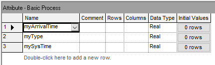
Figure 3.6: Attribute data module
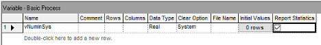
Figure 3.7: Variable data module
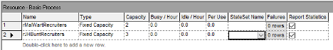
Figure 3.8: Resource data module
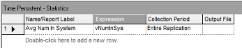
Figure 3.9: Time persistent data module
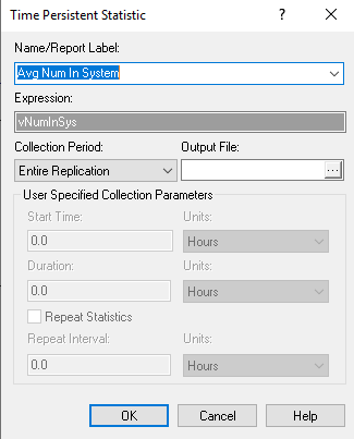
Figure 3.10: Time persistent dialog module view
An example of the Edit by Dialog view is shown in Figure 3.10 for the TIME PERSISTENT module. Notice that every Edit by Dialog view has a Help button that allows easy access to the Arena Help associated with the module. The Arena Help will include information about the text field prompts, the options associated with the module as well as examples and their meaning. The TIME PERSISTENT module requires a name for the statistic being defined as well as an expression that will be observed for statistical collect over time. In this case, the variable, myNumInSys, is used as the expression.
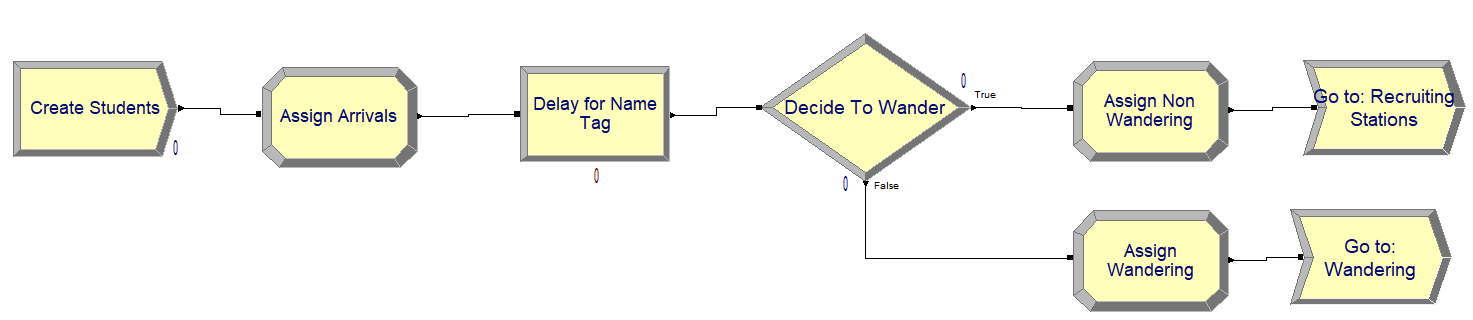
Figure 3.11: Creating students for STEM Career Mixer
Figure 3.11 shows the module layout for creating the students and getting them flowing into the mixer. These modules follow the pseudo-code very closely. Notice in Figure 3.12 the edit by dialog view of the CREATE module is provided. Since we have a Poisson process with rate 0.5 students per minute, the CREATE module is completed in a similar fashion as we discussed in Chapter 2 by specifying the time between arrival process.
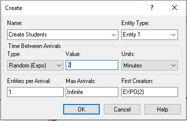
Figure 3.12: CREATE module for STEM Career Mixer
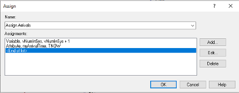
Figure 3.13: ASSIGN arrivals module
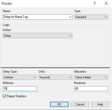
Figure 3.14: DELAY for name tags
Next, Figure 3.13 illustrates the first ASSIGN module, which increments the number of students in the system and assigns the arrival time of the student. Figure 3.14 shows the dialog box for a PROCESS module with the Delay action to implement the delay for putting on the name tag. Notice that this option does not require a resource as we saw in the Chapter 2. We simply need to specify the Delay action and type of the delay with the appropriate distribution (UNIF(15, 45)), in seconds.
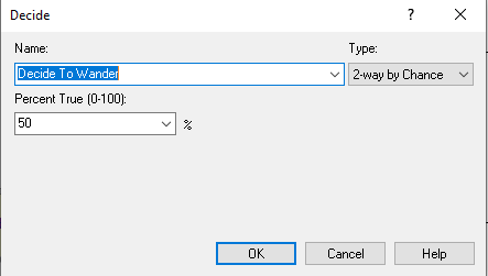
Figure 3.15: DECIDE to wander or not
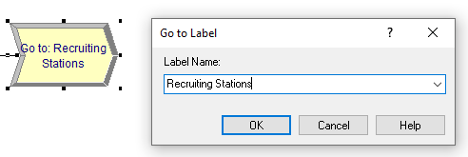
Figure 3.16: GOTO Label: Recruiting Stations
Continuing along with the modules in Figure 3.11, the DECIDE module (shown in Figure 3.15) is used with the 2-way by Chance option, where the branching chance is set at 50%. The two ASSIGN modules simply assign myType to the value 1 (non-wanders) or 2 (wanderers) depending on the result of the random path assignment from the DECIDE with chance option. Finally, we see in Figure 3.16, the GO TO LABEL module, which looks a little like an arrow and simply contains the specified label to where the entity will be directed. In this case, the label is the “Recruiting Stations.”
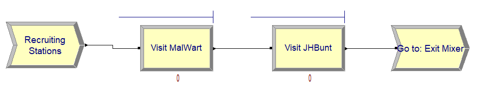
Figure 3.17: Recruiting station process logic
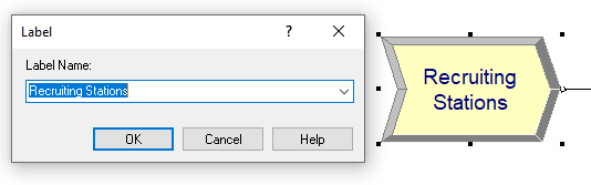
Figure 3.18: Recruiting station label
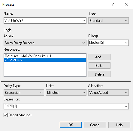
Figure 3.19: Visting MalWart PROCESS module
Figure 3.17 shows the module layout for the recruiting station logic. Notice that Figure 3.18 shows the specification of the label marking the start of the logic. Figure 3.19 show the PROCESS module for the students visiting the MalWart recruiting station. Similar to its use in Chapter 2, this module uses the SEIZE-DELAY-RELEASE option, specifies that the rMalWartRecruiter resource will have one of its two recruiters seized and provides the time delay, EXPO(3) minutes, for the delay time.
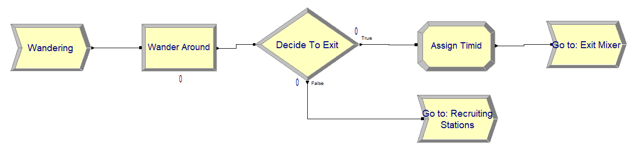
Figure 3.20: Wandering students process logic
Figure 3.20 illustrates the module flow logic for the students that wander. Here, we again use a PROCESS module with the DELAY option, a DECIDE with 2-way by Chance option and GO TO LABEL modules to direct the students. The ASSIGN module in Figure 3.20 simply sets the attribute, myType, to the value 3, as noted in the pseudo-code.
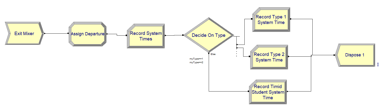
Figure 3.21: Statistics collection exiting logic
Finally, Figure 3.21 presents the model flow logic for collecting statistics when the students leave the mixer. The ASSIGN module of Figure 3.21 is shown in Figure 3.22.
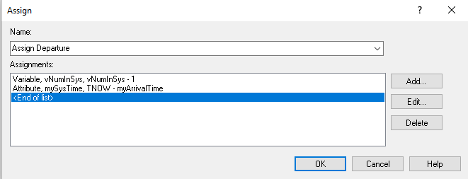
Figure 3.22: ASSIGN module for departures
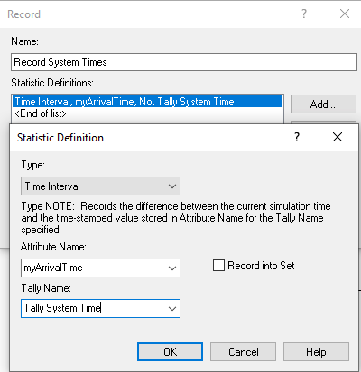
Figure 3.23: RECORD module for system time interval option
In the ASSIGN module, first the number of students in attending the mixer is decremented by 1 and the value of the attribute, mySysTime, is computed. This holds the value of TNOW – myArriveTime, which implements \({T_{i} = D}_{i} - A_{i}\) for each departing student. Figure 3.23 shows the Time Interval option of the RECORD module which, as noted in the dialog box, "Records the difference between the current simulation time and the time-stamped value stored in the Attribute Name for the Tally Name specified." This is, TNOW – myArriveTime, which is the system time.
Since this type of recording is so common the RECORD module provides this option to facilitate this type of collection The RECORD module has five different record types:
- Count
When Count is chosen, the module defines a COUNTER variable. This variable will be incremented or decremented by the value specified.
- Entity Statistics
This option will cause entity statistics to be recorded.
- Time Interval
When Time Interval is chosen, the module will take the difference between the current time, TNOW, and the specified attribute.
- Time Between
When Time Between is chosen, the module will take the difference between the current time, TNOW, and the last time an entity passed through the RECORD module. Thus, this option represents the time between arrivals to the module.
- Expression
The Expression option allows statistics to be collected on a general expression when the entity passes through the module.
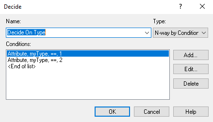
Figure 3.24: DECIDE module for checking type of student
Figure 3.24 shows a DECIDE module with the N-way by Condition option. This causes the DECIDE module to have more than two output path ports. The order of the listed conditions within the module correspond to the output ports on the module. Thus, entities that come out of the first output port have the value of attribute myType equal to 1. The entities entering the DECIDE module must choose one of the paths. Figure 3.25 shows the RECORD module for collection of system time statistics on the entities that have the myType attribute equal to 1. Notice that I have elected to use the Expression option for defining the statistical collection and specified the value of the attribute, mySysTime, as the recorded value. This is the same as choosing the Time Interval option and choosing the myArrivalTime attribute as the time-stamped attribute. This is just another way to accomplish the same task. In fact, the Time Interval option of the RECORD module was invented because this is such a very common modeling task. The rest of the modules in Figure 3.21 are completed in a similar fashion.
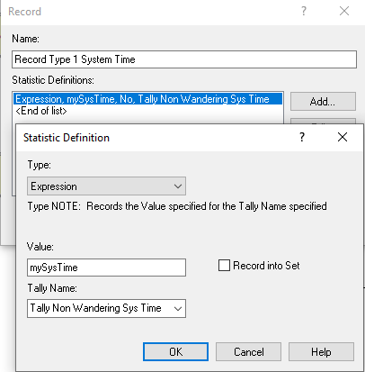
Figure 3.25: Recording statistics on type 1 students
3.4.3 Planning the Sample Size
Now we are ready to run the model and see the results. Figure 3.26 shows the Run Setup configuration to run 5 replications of 6 hours with the base time units in minutes. This means that the simulation will repeat the operation of the STEM mixer 5 times. Each replication will be independent of the others. Thus, we will get a random sample of the operation of 5 STEM mixers over which we can report statistics.
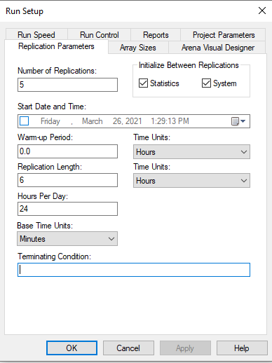
Figure 3.26: Run setup dialog for STEM Mixer example
Running the simulation results in the output for the user defined statistics as show in Figure 3.27. We see that the average system time is 39.192 minutes with a half-width of 9.09 with 95% confidence. Notice also that in Figure 3.27 there are two time-persistent statistics reported for the number of students in the system, both reporting the same statistics. The first one listed is due to our use of the TIME-PERSISTENT module. The second one listed is because, in the VARIABLE module, the report statistic option was checked for the variable vNumInSys. These two approaches result in the same results so using either method is fine. We will see later in the text that using the TIME PERSISTENT module will allow the user to save the collected data to a file and also provides options for collecting statistics over user defined periods of time.
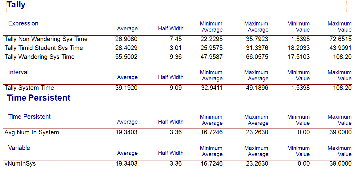
Figure 3.27: STEM Mixer simulation results for 5 replications
Since the STEM mixer organizer wants to estimate the average time students spend at the mixer, regardless of what they do, to be within plus or minus 1 minute with a 95% confidence level, we need to increase the number of replications. To determine the number of replications to use we can use the methods of Section 3.4.1. Noting the initial half-width of \(h_{0} = 9.09\) for \(n_{0} = 5\) replications, the desired half-width, \(h = 1\) minute, and applying Equation (3.12), we have:
\[ n \cong n_{0}\left( \frac{h_{0}}{h} \right)^{2} = 5\left( \frac{9.09}{1} \right)^{2} = 413.14 \approx 414 \]
Updating the number of replications to run to be 414 and executing the model again yields the results in Figure 3.28. We see from Figure 3.28 that the desired half-width criterion of less than 1 minute is met, noting that the resulting half-width is less than 0.79 minutes.
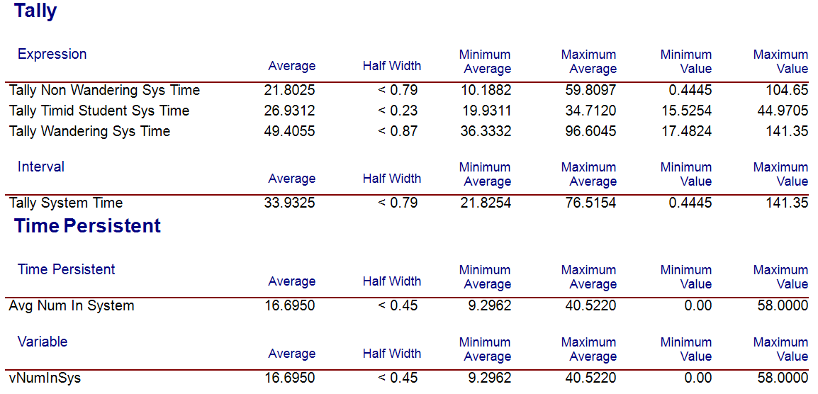
Figure 3.28: STEM Mixer simulation results for 414 replications
To use the Normal approximation method of determining the sample size based on the Arena output, we must first compute the sample standard deviation for the initial pilot sample and then use Equation (3.6):
\[n \geq \left( \frac{z_{1-(\alpha/2)}\;s}{\epsilon} \right)^{2}\]
To compute the sample standard deviation from the half-width, we have:
\[s_{0} = \frac{h_{0}\sqrt{n_{0}}}{t_{1-(\alpha/2),n - 1}} = \frac{9.09 \times \sqrt{5}}{t_{0.975,4}} = \frac{9.09 \times \sqrt{5}}{2.7764} = 7.3208\]
Then, the normal approximation yields:
\[n \geq \left( \frac{z_{1-(\alpha/2)}\;s}{\epsilon} \right)^{2} = \left( \frac{1.9599 \times 7.3208}{1} \right)^{2} = 205.8807 \cong 206 \]
We can also use an iterative approach based on Equation (3.5).
\[ h\left( n \right) = t_{1-(\alpha/2),n - 1}\frac{s(n)}{\sqrt{n}} \leq \varepsilon \] Notice that the equation emphasizes the fact that the half-width, \(h(n)\) and the sample standard deviation, \(s(n)\), both depend on \(n\) in th formula. Using goal-seek within the spreadsheet that accompanies this chapter yields \(n \geq 208.02 =209\) as illustrated in Figure 3.29.
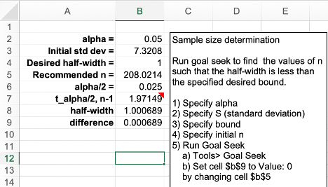
Figure 3.29: Goal Seek Results for Student-t Iterative Method
To summarize, we have the following recommendations for the sample size based on the three methods.
| Method | Recommended Sample Size | Resulting Half-width |
|---|---|---|
| Half-Width Ratio | 414 | < 0.79 |
| Normal Approximation | 206 | < 1.16 |
| Iterative Student T Method | 209 | < 1.18 |
As you can see from the summary in Table 3.3, the methods all result in different recommendations and different resulting half-widths. Why are the recommendations different? Because each method makes different assumptions. In addition, you must remember that the results shown here are based on an initial pilot run of 5 samples. Using a larger initial pilot sample size will result in different recommendations. Running the model for 10 replications yields an initial half-width of 5.4 minutes and the recommendations in Table 3.4.
| Method | Recommended Sample Size | Resulting Half-width |
|---|---|---|
| Half-Width Ratio | 292 | < 0.96 |
| Normal Approximation | 219 | < 1.14 |
| Iterative Student T Method | 221 | < 1.14 |
Based on these results, we can be pretty certain that the number of replications needed to get close to 1 minute half-width with 95% confidence is somewhere between 219 and 292. So, which method should you use? Generally, the half-width ratio method is the most conservative of the approaches and will recommend a larger sample size.
Why does determining the sample size matter? This model takes less than a second per replication. But what if a single replication required 1 hour of execution time. Then, we will really care about determining to the extent possible the minimum number of samples needed to provide a result upon which we can make a confident decision. Thus, there is a trade-off between the time needed to get a result and the desired precision of the result. This trade-off motivates the use of sequentially sampling until the desired half-width is met. This is the topic of the next section.