4.7 Modeling Systems with Routing Sequences
A network of queues can be thought of as a set of stations, where each station represents a service facility. In the simple case, each service facility might have a single queue feeding into a resource. In the most general case, customers may arrive to any station within the network from outside the system. Customers then proceed from station to station to receive service. After receiving all of their service requirements, the customers depart the system.
In general the customers, do not take the same path through the network and for a given customer type, the path may be deterministic or stochastic in nature. For example, consider the case of a job shop manufacturing setting. Each product that is manufactured may require a different set of manufacturing processes, which are supplied by particular stations (e.g. drilling, milling, etc.). As another example, consider a telecommunications network where packets are sent from some origin to some destination through a series of routers. In each of these cases, understanding how many resources to supply so that the customer can efficiently traverse the network at some minimum cost is important. As such, queuing networks are an important component of the efficient design of manufacturing, transportation, distribution, telecommunication, computer, and service systems. Figure 4.93 illustrates the concept of a network of stations for producing a vacuum cleaner.
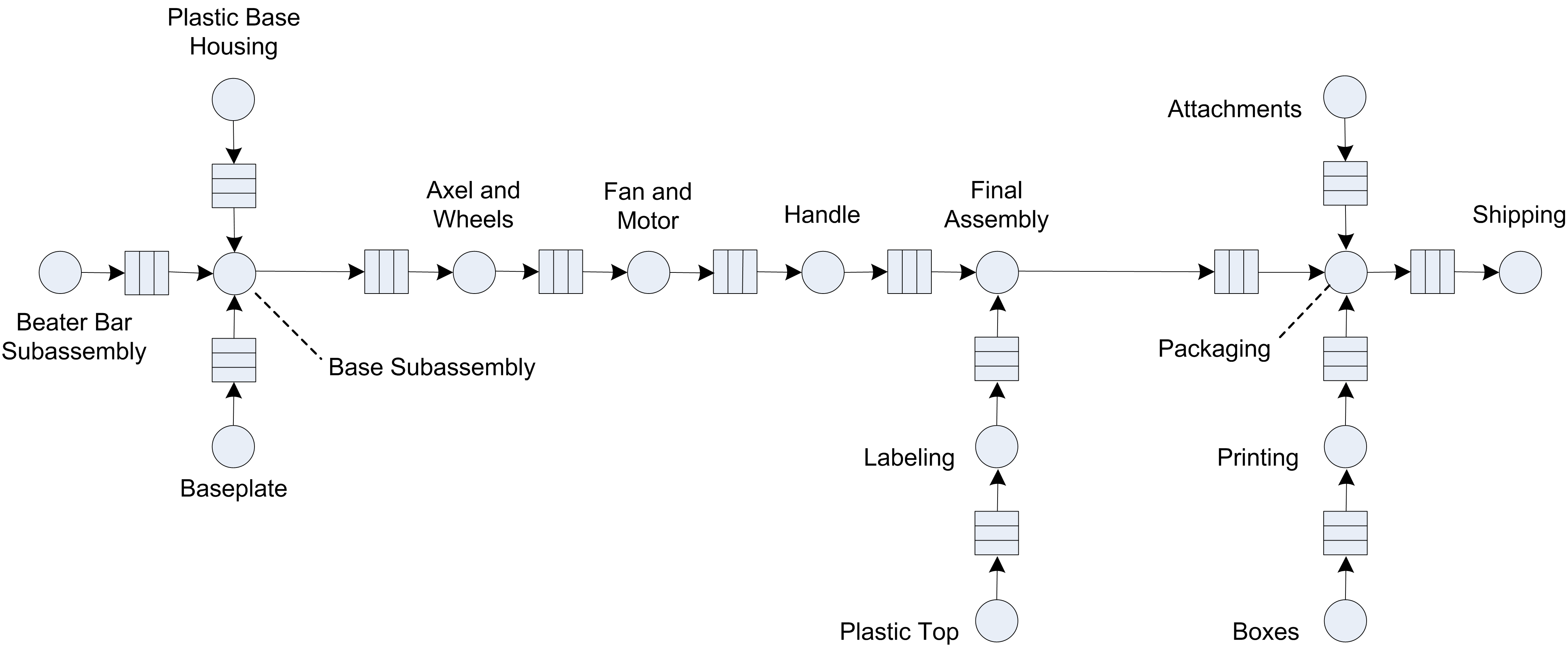
Figure 4.93: Vaccum cleaner manufacturing system as a network of stations
The analytical treatment of the theory associated with networks of queues has been widely examined and remains an active area for theoretical research. It is beyond the scope of this text to discuss the enormous literature on queuing networks. The interested reader is referred to the following texts as a starting point, (Gross and Harris 1998), (Kelly 1979), (Buzacott and Shanthikumar 1993), or Bolch et al. (2006).
A number of examples have already been examined that can be considered queuing networks (e.g. the Tie-Dye T-Shirts and the LOTR’s Ring Making examples). The purpose of this section will be to introduce some constructs that facilitate the simulation of queuing networks. Since a queuing network involves the movement of entities between stations, the use of the STATION, ROUTE, and SEQUENCE modules from the Advanced Transfer template panel will be emphasized.
4.7.1 Computer Test and Repair Shop Example
Consider a test and repair shop for computer parts (e.g. circuit boards, hard drives, etc.) The system consists of an initial diagnostic station through which all newly arriving parts must be processed. Currently, newly arriving parts arrive according to a Poisson arrival process with a mean rate of 3 per hour. The diagnostic station consists of 2 diagnostic machines that are fed the arriving parts from a single queue. Data indicates that the diagnostic time is quite variable and follows an exponential distribution with a mean of 30 minutes. Based on the results of the diagnostics, a testing plan is formulated for the parts. There are currently three testing stations 1. 2, 3 which consist of one machine each. The testing plan consists of an ordered sequence of testing stations that must be visited by the part prior to proceeding to a repair station. Because the diagnosis often involves similar problems, there are common sequences that occur for the parts. The company collected extensive data on the visit sequences for the parts and found that the sequences in Table 4.3 constituted the vast majority of test plans for the parts.
| Test Plan | % of Parts | Sequence |
|---|---|---|
| 1 | 25% | 2,3,2,1 |
| 2 | 12.5% | 3,1 |
| 3 | 37.5% | 1,3,1 |
| 4 | 25% | 2,3 |
For example, 25% of the newly arriving parts follow test plan 1, which consists of visiting test stations 2, 3, 2, and 1 prior to proceeding to the repair station.
The testing of the parts at each station takes time that may depend upon the sequence that the part follows. That is, while parts that follow test plan’s 1 and 3 both visit test station 1, data shows that the time spent processing at the station is not necessarily the same. Data on the testing times indicate that the distribution is well modeled with a lognormal distribution with mean, \(\ \mu\), and standard deviation, \(\sigma\) in minutes. Table 4.4 presents the mean and standard deviation for each of the testing time distributions for each station in the test plan.
| Test Plan | Testing Time Parameters | Repair Time Parameters |
|---|---|---|
| 1 | (20,4.1), (12,4.2), (18,4.3), (16,4.0) | (30,60,80) |
| 2 | (12,4), (15,4) | (45,55,70) |
| 3 | (18,4.2), (14,4.4), (12,4.3) | (30,40,60) |
| 4 | (24,4), (30,4) | (35,65,75) |
For example, the first pair of parameters, (20, 4.1), for test plan 1 indicates that the testing time at test station 2 has a lognormal distribution with mean,\(\mu = 20\), and standard deviation,\(\sigma = 4.1\) minutes.
The repair station has 3 workers that attempt to complete the repairs based on the tests. The repair time also depends on the test plan that the part has been following. Data indicates that the repair time can be characterized by a triangular distribution with the minimum, mode, and maximum as specified in the previous table. After the repairs, the parts leave the system. When the parts move between stations assume that there is always a worker available and that the transfer time takes between 2 to 4 minutes uniformly distributed. Figure 4.94 illustrates the arrangement of the stations and the flow of the parts following Plan 2 in the test and repair shop.
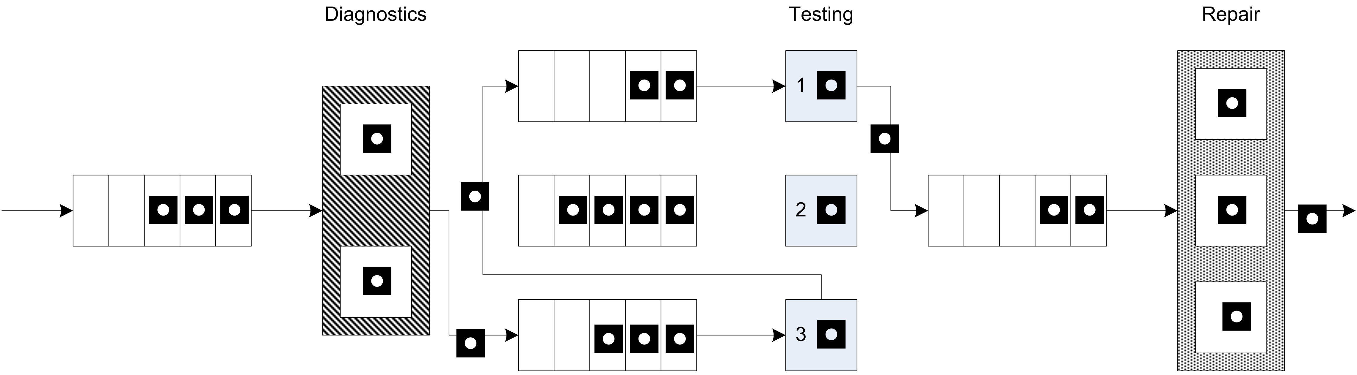
Figure 4.94: Overview of the test and repair shop
The company is considering accepting a new contract that will increase the overall arrival rate of jobs to the system by 10%. They are interested in understanding where the potential bottlenecks are in the system and in developing alternatives to mitigate those bottlenecks so that they can still handle the contract. The new contract stipulates that 80% of the time the testing and repairs should be completed within 480 minutes. The company runs 2 shifts each day for each 5 day work week. Any jobs not completed at the end of the second shift are carried over to first shift of the next working day. Assume that the contract is going to last for 1 year (52 weeks). Build a simulation model that can assist the company in assessing the risks associated with the new contract.
4.7.2 Conceptualizing the Model
Before implementing the model, you should prepare by conceptualizing the process flow. Figure 4.95 illustrates the activity diagram for the test and repair system. Parts are created and flow first to the diagnostic station where they seize a diagnostic machine while the diagnostic activity occurs. Then, the test plan is assigned. The flow for the visitation of the parts to the test station is shown with a loop back to the transfer time between the stations. It should be clear that the activity diagram is representing any of the three test stations. After the final test station in the test plan has been visited, the part goes to the repair station, where 1 of 3 repair workers is seized for the repair activity. After the repair activity, the part leaves the system.
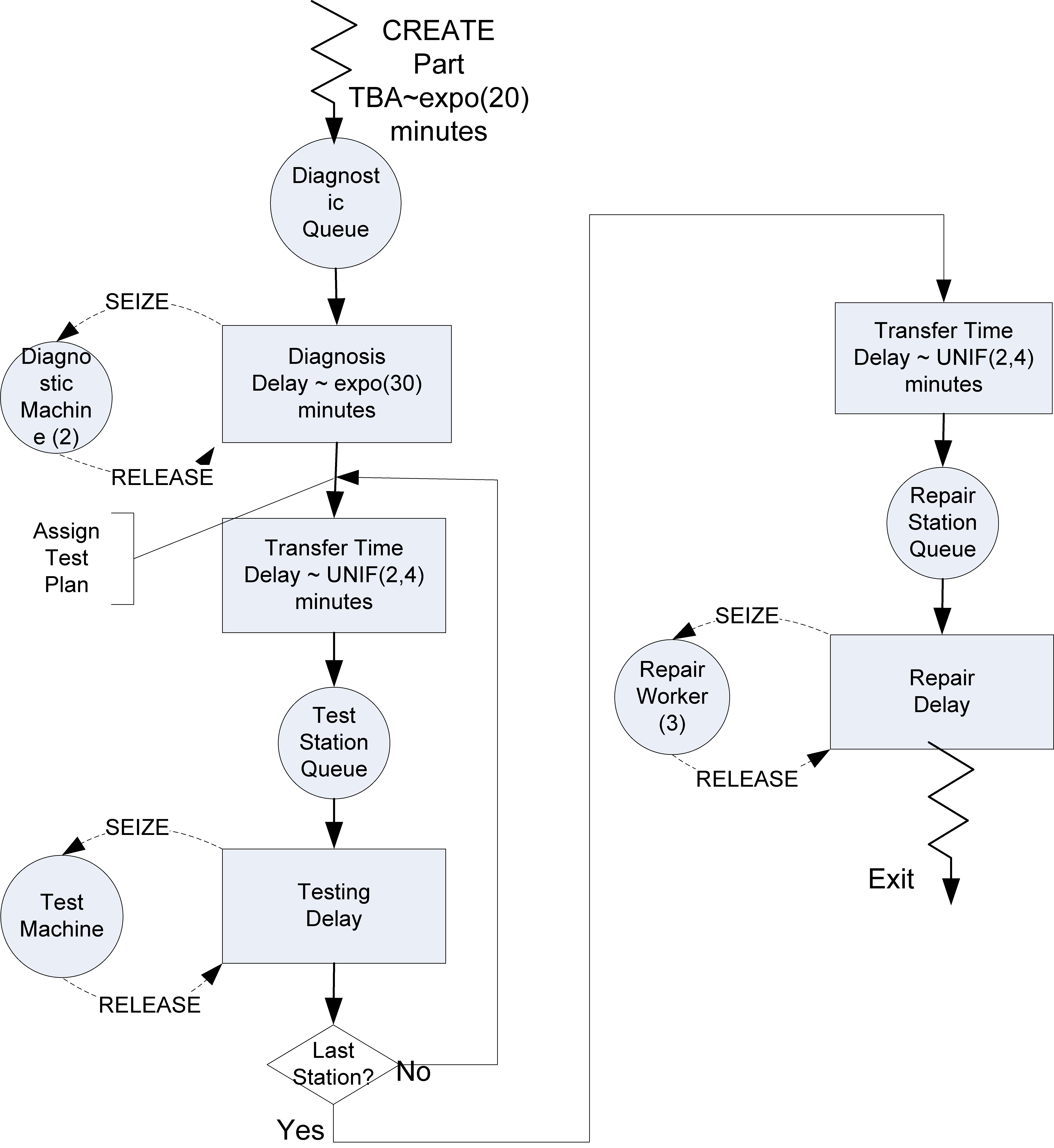
Figure 4.95: Activity diagram for test and repair system
The following pseudo-code represent the main concepts for modeling the test and repair system. This is a straight forward representation of the flow presented in the activity diagram. From the activity diagram and the pseudo-code, it should be clear that with the current modeling constructs you should be able to model this situation. In order to model the situation, you need some way to represent where the part is currently located in the system (e.g. the current station). Secondly, you need some way to indicate where the part should go to next. And finally, you need some way to model the transfer and the time of the transfer of the part between stations. This type of modeling is very common. Because of this, there are special modules that are specifically designed to handle situations like this.
CREATE part
BEGIN PROCESS Diagnostics
    SEIZE 1 diagnostic machine
    DELAY for diagnostic time
    RELEASE diagnostic machine
END PROCESS
BEGIN ASSIGN
    determine test plan type
    determine SEQUENCE for test plan type
END ASSIGN
ROUTE for transfer time by SEQUENCE to STATION Test

STATION Test
BEGIN PROCESS Testing
    SEIZE appropriate test machine
    DELAY for testing time
    RELEASE test machine
END PROCESS
DECIDE IF not at last station
        ROUTE for transfer time by SEQUENCE to STATION Test
ELSE
        ROUTE for transfer time by SEQUENCE to STATION Repair
END DECIDE

STATION Repair
BEGIN PROCESS Repair Process
    SEIZE repair worker from repair worker set
    DELAY for repair time
    RELEASE repair worker
END PROCESS
RECORD statistics
DISPOSE
The pseudo-code introduces some new concepts involving sequences, routes, and stations. The next section introduces these very useful constructs.
4.7.3 STATION, ROUTE, and SEQUENCE Modules
Entities typically represent the things that are flowing through the system. Entity transfer refers to the various ways by which entities can move between modules. As we have previously seen, the STATION and ROUTE modules facilitate the transfer of entities between stations with a transfer delay. The SEQUENCE module defines a list of stations to be visited.
- SEQUENCE
The SEQUENCE module is a data module that defines an ordered list of stations. The list represents the natural order in which the stations will be visited, if transferred using the ROUTE module with the By Sequence option. In addition to defining a list of stations, a SEQUENCE permits the listing of a set of assignments (e.g. ASSIGN modules) to be executed when the transfer occurs.
Unlike our previous use of the STATION and ROUTE module, we may need to know where (at which station) the entities are in order to provide appropriate processing logic. Entities have a number of special purpose attributes that are useful
when modeling with the SEQUENCE, STATION, and ROUTE modules. The
Entity.Station and Entity.CurrentStation keep track of the location
of the entity within the model. The attribute, Entity.CurrentStation
is updated to the current station whenever the entity passes through the
STATION module. This attribute is not user assignable, but can be used
(read) in the model. It will return the station number for the current
station of the entity or 0 if the entity is not currently at a station.
In addition, every entity has an Entity.Station attribute, which
returns the entity’s station or destination. The Entity.Station
attribute is user assignable. It is (automatically) set to the intended
destination station when an entity is transferred (e.g. via a ROUTE
module). It will remain equal to the current station after the transfer
or until either changed by the user or affected by another transfer type
module (e. g. ROUTE module). Thus, the modules attached to a STATION
module are conceptually at the station location.
In many modeling contexts, entities will follow a specific path through the system. In a manufacturing job shop, this is often called the process plan. In a bus system, this called a bus route. In the test and repair system, this is referred to as the test plan. To model a specify path through the system, the SEQUENCE module can be used. A sequence consists of an ordered list of job steps. Each job step must indicate the STATION associated with the step and may indicate a series of assignments that must take place when the entity reaches the station associated with the job step. Each job step can have an optional name and can give the name of the next step in the sequence. Thus, a sequence is built by simply providing the list of stations that must be visited.
Each entity has a number of special purpose attributes that facilitate
the use of sequences. The Entity.Sequence attribute holds the sequence
that the entity is currently following or 0 if no sequence has been
assigned. The ASSIGN module can be used to assign a specific sequence to
an entity. In addition, the entity has the attribute, Entity.JobStep,
which indicates the current step within the sequence that the entity is
executing. Entity.JobStep is user assignable and is automatically
incremented when a transfer type module (e.g. ROUTE) is used with the
By Sequence option. Finally, the attribute (Entity.PlannedStation)
is available and represents the number of the station associated with
the next job step in the sequence. Entity.PlannedStation is not
user-assignable. It is automatically updated whenever Entity.Sequence
or Entity.JobStep changes, or whenever the entity enters a station.
In the test and repair example, STATION modules will be associated with
the diagnostic station, each of three test stations, and with the repair
station. The work performed at each station will be modeled with a
PROCESS module using the (SEIZE, DELAY, and RELEASE) option. The four
different test plans will be modeled with four sequences. Finally, ROUTE
modules, using the By Sequence transfer option will be used to
transfer the entities between the stations with a UNIF(2,4) transfer
delay time distribution in minutes. Other than the new modules for
entity transfer this model is similar to previous models. This model can
be built by following these steps:
Define 5 different resources (
DiagnosticMachine,TestMachine1,TestMachine2,TestMachine3,RepairWorkers) with capacity (2, 1, 1, 1, 3) respectively.Define 2 variables (
vContractLimit,vMTBA) with initial values (480 and 20) respectively. These variables represent the length of the contract and the mean time between arrivals, respectively.Define 3 expressions (
eDiagnosticTime,eTestPlanCDF, andeRepairTimeCDFs).eDiagnosticTimeshould be expo(30),eTestPlanCDFshould be DISC(0.25, 1, 0.375, 2, 0.75,3, 1.0,4). In this distribution 1, 2, 3, 4 represents the four test plans. Finally,eRepairTimeCDFsshould be an arrayed expression with four rows. Each row should specify a triangular distribution according to the information given concerning the repair time distributions (e.g. TRIA(30,60,80).Use the SEQUENCE module on the Advanced Transfer panel to define four different sequences. This is illustrated in Figure 4.96. First, double click on the SEQUENCE module to add a new sequence (row). The first sequence is called
TestPlan1Seq.Then, add job steps to the sequence by clicking on the Steps button. Figure 4.96 shows the five job steps for test plan 1 (TestStation2,TestStation3,TestStation2,TestStation1, andRepairStation). Typing in a station name defines a station for use in the model window. Since every part must visit the repair station before exiting the system,RepairStationhas been listed last in all the sequences.For each job step, define an assignment that will happen when the entity is transferred to the step. In the test and repair system, the testing time depends upon the job step. Thus, an attribute,
myTestingTime, can be defined so that the value from the pertinent lognormally distributed test time distribution can be assigned. In the case illustrated,myTestingTimewill be set equal to a random number from a LOGN(20, 4.1) distribution, which represents the distribution for test station 2 on the first test plan. ThemyTestingTimeattribute is used to specify the delay time for each of the PROCESS modules that represent the testing processes.Finally, define a set to hold the sequences so that they can be randomly assigned to the parts after they visit the diagnostic machine. To define a Sequence set, you must use the Advance Set module on the Advance Process panel. Each of the sequences should be listed in the set as shown in Figure 4.97. The set type should be specified as Other. Unfortunately, the build expression option is not available here and each sequence name must be carefully typed into the dialog box. The order of the sequences is important.
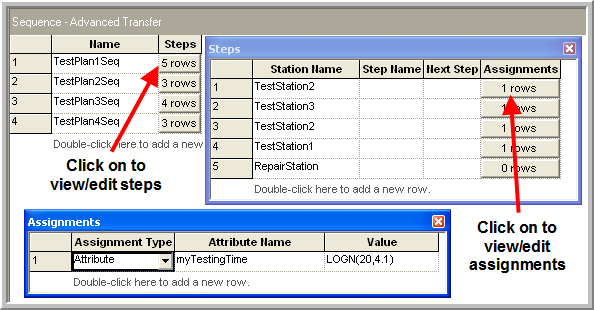
Figure 4.96: Defining sequences, job steps, and assignments
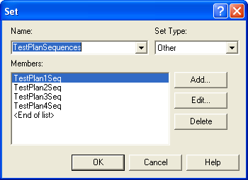
Figure 4.97: Defining an advanced set to hold the sequences
Now that all the data modules have been specified, you can easily build
the model using the flow chart modules. The completed model can be found in the book support files associated with chapter called, RepairShop.doe. Figure 4.98 presents an overview of the model. The
pink colored modules in the figure are the STATION and ROUTE modules. A
CREATE module is used to generate the parts needing testing and repair
with a mean time between arrivals of 20 minutes exponentially
distributed. Then, the entity proceeds through an ASSIGN module where
the attribute, myArriveTime, is set to TNOW. This will be used to
record the job’s system time. The next module is a STATION module that
represents the diagnostic station, see
Figure 4.99.

Figure 4.98: Overview of the test and repair model
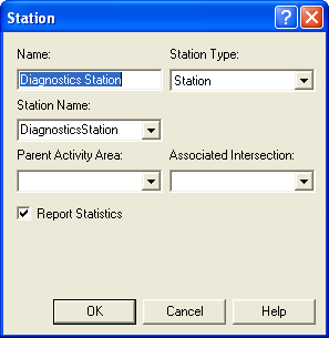
Figure 4.99: Modeling the diagnostics station with a STATION module
After passing through the STATION module, the entity goes through the
diagnostic process. Following the diagnostic process, the part is
assigned a test plan.
Figure 4.100 shows that the test plan expression holding
the DISC distribution across the test plans is used to assign a number
1, 2, 3, or 4 to the attribute myTestPlan. Then, the attribute is used
to select the appropriate sequence from our previously defined set of
test plan sequences. The sequence returned from the set is assigned to
the special purpose attribute, Entity.Sequence, so that the entity can
now follow this sequence.
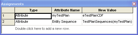
Figure 4.100: Assigning the test plans
The part then enters the ROUTE module for sending the parts to the
testing stations. Figure 4.101 illustrates the ROUTE module. This module allows a time delay in the route time field and allows the user to
select the method by which the entity will be transferred. Choosing the
By Sequence option indicates that the entity should use its assigned
sequence (via the Entity.Sequence attribute) to determine the
destination station for the route. The entity’s sequence and its current
job step are used. When the entity goes into the ROUTE module,
Entity.JobStep is incremented to the next step. The entity’s
Entity.Station attribute is set equal to the station associated with
the step and all attributes associated with the step are executed. Then,
the entity is transferred (starts the delay associated with the
transfer). After the entity completes the transfer and enters the
destination station, the entity’s Entity.CurrentStation attribute is
updated.
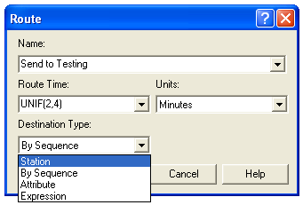
Figure 4.101: Selecting the By Sequence option within the ROUTE module
In the example, the part is sent to the appropriate station on its
sequence. Each of the stations used to represent the testing stations
follow the same pattern (STATION, PROCESS (seize, delay, release), and
ROUTE). The PROCESS module (Figure 4.102) uses the attribute, myTestingTime, to
determine the delay time for the testing process. This attribute was set
when the entity’s job step attributes were executed.
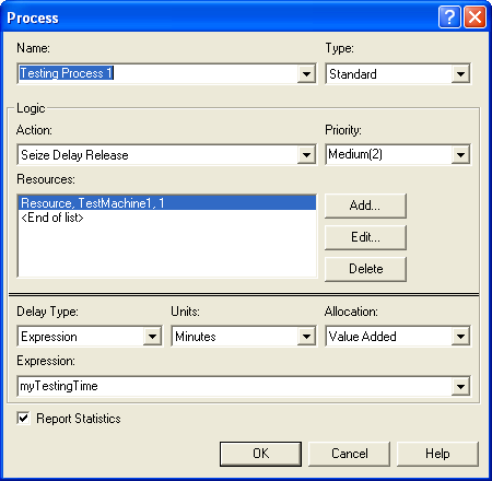
Figure 4.102: PROCESS module for the testing process
After proceeding through its testing plan, the part is finally routed to
the RepairStation, since it was the station associated with the last
job step. At the repair station, the part goes through its repair
process by using the expression eRepairTimeCDFs and its attribute,
myTestPlan, as shown in Figure 4.103.
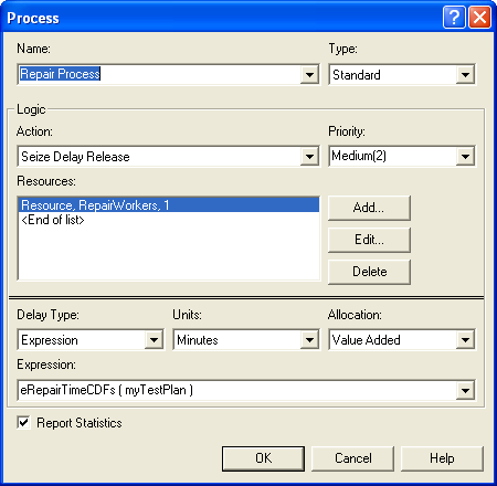
Figure 4.103: PROCESS module for the repair process
The ASSIGN module after the repair process module simply computes the
entity’s total system time in the attribute, mySysTime, so that the
following two RECORD modules can compute the appropriate statistics as
indicated in Figure 4.104.
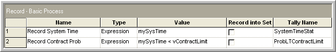
Figure 4.104: RECORD modules for test and repair model
4.7.4 Running the Test and Repair Model
Now the model is ready to set up and run. According to the problem, the purpose of the simulation is to evaluate the risk associated with the contract. The life of the contract is specified as 1 year (52 weeks \(\times\) 5 days/week \(\times\) 2 shifts/day \(\times\) 480 minutes/shift = 249,600 minutes). Since the problem states that any jobs not completed at the end of a shift are carried over to the next working day, it is as if there are 249,600 minutes or 4,160 hours of continuous operation available for the contract. This is also a terminating simulation since performance during the life of the contract is the primary concern. The only other issue to address is how to initialize the system. The analysis of the two situations (current contract versus contract with 10% more jobs) can be handled via a relative comparison. Thus, to perform a relative comparison you need to ensure that both alternatives start under the same initial conditions. For simplicity, assume that the test and repair shop starts each contract alternative under empty and idle conditions. Let’s assume that 10 replications of 4,160 hours will be sufficient as illustrated in Figure 4.105.
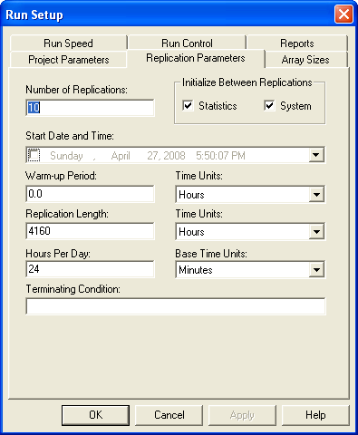
Figure 4.105: Run setup specification for test and repair shop model
As shown in Figure 4.106, for the current situation, the probability that a job completes its testing and repair within 480 minutes is about 82%. The addition of more jobs should increase the risk of not meeting the contract specification. You are asked to analyze the new contract’s risks and make a recommendation to the company on how to proceed within the exercises.
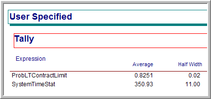
Figure 4.106: User defined statistics for current contract
In the test and repair example, the time that it took to transfer the parts between the stations was a simple stochastic delay (e.g. UNIF (2,4) minutes). The STATION, ROUTE, and SEQUENCE modules make the modeling of entity movement between stations in this case very straightforward. In some systems, the modeling of the movement is much more important because material handling devices (e.g. people to carry the parts, fork lifts, conveyors, etc.) may be required during the transfer. These will require an investigation of the modules within the Advanced Transfer Panel. This topic will be taken up in Chapter 7.